<?xml version="1.0" encoding="utf-8"?><feed xmlns="http://www.w3.org/2005/Atom" ><generator uri="https://jekyllrb.com/" version="3.10.0">Jekyll</generator><link href="https://girijesh-ai.github.io/feed.xml" rel="self" type="application/atom+xml" /><link href="https://girijesh-ai.github.io/" rel="alternate" type="text/html" /><updated>2026-02-20T14:11:36+00:00</updated><id>https://girijesh-ai.github.io/feed.xml</id><title type="html">Girijesh Prasad’s AI Blog</title><subtitle>Deep dives into AI, Machine Learning, and Agentic Systems. Practical guides for AI Engineers and Data Scientists.</subtitle><author><name>Girijesh Prasad</name><email>girijeshprasad@example.com</email></author><entry><title type="html">The Story of Embedding — Deep Dive: From Bag of Words to Sentence Transformers</title><link href="https://girijesh-ai.github.io/ai/llm/embedding/2026/02/20/story-of-embedding.html" rel="alternate" type="text/html" title="The Story of Embedding — Deep Dive: From Bag of Words to Sentence Transformers" /><published>2026-02-20T03:30:00+00:00</published><updated>2026-02-20T03:30:00+00:00</updated><id>https://girijesh-ai.github.io/ai/llm/embedding/2026/02/20/story-of-embedding</id><content type="html" xml:base="https://girijesh-ai.github.io/ai/llm/embedding/2026/02/20/story-of-embedding.html"><![CDATA[<h1 id="the-story-of-embedding--deep-dive-from-bag-of-words-to-sentence-transformers">The Story of Embedding — Deep Dive: From Bag of Words to Sentence Transformers</h1>

<p><em>The mathematical intuitions, architectural decisions, and production lessons behind 70 years of teaching machines to understand language.</em></p>

<hr />

<h2 id="why-this-post-exists">Why This Post Exists</h2>

<p>There are hundreds of “intro to embeddings” posts out there. Most of them tell you <em>what</em> Word2Vec and BERT are. Very few explain <em>why</em> each generation of embeddings emerged, what mathematical insight drove each breakthrough, and what actually matters when you’re deploying these systems in production.</p>

<p>This post is for engineers who want to go deeper — who want to understand not just the “what” but the “why” and the “how it actually works under the hood.”</p>

<p>Let’s trace the full arc, starting from first principles.</p>

<hr />

<h2 id="1-the-representation-problem-why-vectors">1. The Representation Problem: Why Vectors?</h2>

<p>Before we count a single word, we need to answer a fundamental question: <strong>why represent text as vectors at all?</strong></p>

<p>The answer is deceptively simple: <strong>vectors give us geometry</strong>, and geometry gives us the ability to <em>measure</em>. Once you have text as vectors, you can compute distances (how different are two documents?), find nearest neighbours (what’s the most similar sentence?), and perform operations (what’s halfway between “happy” and “sad”?).</p>

<p>The entire history of embeddings is really the history of making these geometric operations <em>meaningful</em> — making the geometry of the vector space mirror the semantics of language.</p>

<pre class="mermaid">
timeline
    title The Evolution of Text Embeddings
    section Count-Based
        1950s : Bag of Words
            : Simple frequency counting
        1990 : LSA (SVD)
            : Latent semantic structure
        1992 : TF-IDF
            : Information-theoretic weighting
    section Neural Static
        2003 : Bengio NPLM
            : First neural word embeddings
        2013 : Word2Vec
            : Negative sampling breakthrough
        2014 : GloVe
            : Global co-occurrence factorisation
        2016 : FastText
            : Subword n-grams
    section Contextual
        2017 : Transformer
            : Self-attention architecture
        2018 : ELMo
            : Layer-wise contextual representations
        2018 : BERT
            : Pretraining-finetuning paradigm
    section Sentence-Level
        2019 : Sentence-BERT
            : Siamese bi-encoders
        2020 : ColBERT
            : Late interaction
        2022 : Matryoshka
            : Adaptive dimensionality
        2023-24 : E5 / BGE / NV-Embed
            : Instruction-tuned embeddings
</pre>

<hr />

<h2 id="2-the-counting-era-bow-tf-idf-and-their-hidden-mathematics">2. The Counting Era: BoW, TF-IDF, and Their Hidden Mathematics</h2>

<h3 id="bag-of-words-1950s">Bag of Words (1950s)</h3>

<table>
  <tbody>
    <tr>
      <td>BoW maps each document to an</td>
      <td>V</td>
      <td>-dimensional vector, where</td>
      <td>V</td>
      <td>is the vocabulary size. Simple frequency counting. But here’s what most tutorials skip: <strong>BoW is actually performing a projection from the infinite-dimensional space of possible utterances onto a finite vector space</strong> — and it’s a lossy projection that discards word order, syntax, and semantics.</td>
    </tr>
  </tbody>
</table>

<table>
  <tbody>
    <tr>
      <td>The fundamental limitation isn’t just “no semantics.” It’s the <strong>curse of dimensionality for sparse vectors</strong>. With</td>
      <td>V</td>
      <td>= 100,000, every document lives in a 100,000-dimensional space where cosine similarity becomes almost meaningless — in high-dimensional sparse spaces, all pairwise distances converge, a phenomenon known as the <strong>concentration of measure</strong>.</td>
    </tr>
  </tbody>
</table>

<h3 id="tf-idf-information-theoretic-weighting">TF-IDF: Information-Theoretic Weighting</h3>

<p>TF-IDF is more interesting than most people realise. The IDF component:</p>

\[\text{IDF}(t) = \log\frac{N}{df(t)}\]

<p>is essentially an <strong>information-theoretic</strong> quantity. A word that appears in every document (df(t) = N) has IDF = 0 — zero information value. A rare word has high IDF. This connects directly to Shannon’s self-information: rare events carry more information.</p>

<p>But TF-IDF still builds on the <strong>independence assumption</strong> — it treats each word as statistically independent of every other word. “New York” is just “New” + “York”. This is where the paradigm needed to break.</p>

<h3 id="lsa-the-forgotten-bridge-1990">LSA: The Forgotten Bridge (1990)</h3>

<p>Most “embedding history” posts jump from TF-IDF to Word2Vec, skipping the critical intermediate step: <strong>Latent Semantic Analysis (LSA)</strong> by Deerwester et al. (1990).</p>

<p>LSA takes the term-document matrix and applies <strong>Singular Value Decomposition (SVD)</strong>:</p>

\[X \approx U_k \Sigma_k V_k^T\]

<p>By keeping only the top-k singular values, you project documents into a k-dimensional space (typically k=100-300) where <strong>synonyms collapse together</strong> and <strong>polysemy partially resolves</strong>. LSA was the first demonstration that <strong>dimensionality reduction on co-occurrence data captures latent semantic structure</strong>.</p>

<p>This insight — that meaning hides in the statistical structure of co-occurrence — is the intellectual ancestor of everything that follows.</p>

<hr />

<h2 id="3-the-neural-turn-bengios-nplm-2003--the-forgotten-origin">3. The Neural Turn: Bengio’s NPLM (2003) — The Forgotten Origin</h2>

<p>The standard narrative says Word2Vec (2013) started neural embeddings. <strong>That’s wrong.</strong> The actual origin is Yoshua Bengio’s <strong>Neural Probabilistic Language Model (NPLM)</strong>, published in 2003 — a full decade earlier.</p>

<p>Bengio’s key insight: assign each word a <strong>learned distributed representation</strong> (a dense vector), then train a neural network to predict the next word from the concatenation of the previous n words’ vectors.</p>

<p>The model had three components:</p>

<ol>
  <li>
    <table>
      <tbody>
        <tr>
          <td><strong>Embedding lookup table</strong> C: a</td>
          <td>V</td>
          <td>× d matrix mapping word indices to d-dimensional vectors</td>
        </tr>
      </tbody>
    </table>
  </li>
  <li><strong>Hidden layer</strong>: <code class="language-plaintext highlighter-rouge">h = tanh(H · [C(w_{t-n+1}); ...; C(w_{t-1})] + b)</code></li>
  <li>
    <table>
      <tbody>
        <tr>
          <td><strong>Output softmax</strong>: probability distribution over all</td>
          <td>V</td>
          <td>words</td>
        </tr>
      </tbody>
    </table>
  </li>
</ol>

<p>The genius was that the <strong>embedding table C was learned jointly</strong> with the prediction task. Words that could appear in similar contexts would naturally get similar embeddings, because similar embeddings would produce similar predictions through the hidden layer.</p>

<pre class="mermaid">
graph LR
    subgraph Input["Input: Previous n words"]
        W1["w(t-3)"] --&gt; E1["Embedding C(w(t-3))"]
        W2["w(t-2)"] --&gt; E2["Embedding C(w(t-2))"]
        W3["w(t-1)"] --&gt; E3["Embedding C(w(t-1))"]
    end
    E1 --&gt; CONCAT["Concatenate"]
    E2 --&gt; CONCAT
    E3 --&gt; CONCAT
    CONCAT --&gt; HIDDEN["Hidden Layer - tanh Hx + b"]
    HIDDEN --&gt; SOFTMAX["Softmax over V words - O(V) bottleneck"]
    SOFTMAX --&gt; PRED["P w_t = next word"]
    style SOFTMAX fill:#ff6b6b,stroke:#333,color:#fff
    style PRED fill:#51cf66,stroke:#333,color:#fff
</pre>

<table>
  <tbody>
    <tr>
      <td><strong>Why did it take 10 years to become mainstream?</strong> Bengio’s model was computationally expensive. The softmax output layer required computing a</td>
      <td>V</td>
      <td>-way classification <em>for every position in the training data</em>. With V = 100K words and billions of training positions, this was intractable in 2003.</td>
    </tr>
  </tbody>
</table>

<p>Word2Vec’s real contribution wasn’t the idea of neural embeddings — it was making them <strong>computationally feasible</strong>.</p>

<hr />

<h2 id="4-word2vec-2013-the-trick-was-in-the-training">4. Word2Vec (2013): The Trick Was in the Training</h2>

<h3 id="the-skip-gram-objective">The Skip-gram Objective</h3>

<p>Skip-gram’s true objective function maximises:</p>

\[J = \frac{1}{T} \sum_{t=1}^{T} \sum_{-c \leq j \leq c, j \neq 0} \log P(w_{t+j} | w_t)\]

<p>where T is the total words in the corpus, c is the context window size, and:</p>

\[P(w_O | w_I) = \frac{\exp(\tilde{v}_{w_O}^{\,T} \cdot v_{w_I})}{\sum_{w=1}^{V} \exp(\tilde{v}_w^{\,T} \cdot v_{w_I})}\]

<p>The denominator is a <strong>sum over the entire vocabulary</strong> — this is the bottleneck that killed Bengio’s model. With V = 100K+, computing this for every training example is absurdly expensive.</p>

<h3 id="negative-sampling-the-actual-innovation">Negative Sampling: The Actual Innovation</h3>

<p>Mikolov’s key contribution was <strong>negative sampling</strong>, which replaces the expensive softmax with a much cheaper binary classification:</p>

\[\log \sigma(\tilde{v}_{w_O}^{\,T} \cdot v_{w_I}) + \sum_{i=1}^{k} \mathbb{E}_{w_i \sim P_n(w)} [\log \sigma(-\tilde{v}_{w_i}^{\,T} \cdot v_{w_I})]\]

<p>Instead of computing probabilities over all V words, you:</p>

<ol>
  <li>Take the actual context word (positive) — push its vector <strong>towards</strong> the target</li>
  <li>Sample k random “noise” words (negatives, typically k=5-15) — push their vectors <strong>away</strong> from the target</li>
</ol>

<p>The noise distribution P_n(w) is the unigram distribution raised to the 3/4 power: <code class="language-plaintext highlighter-rouge">P_n(w) = U(w)^{3/4}/Z</code>. The 3/4 exponent is an empirical choice that slightly upweights rare words relative to their frequency — preventing extremely common words from dominating the negative samples.</p>

<p>This reduced training from O(V) per example to O(k) per example. <strong>That’s the real reason Word2Vec succeeded where Bengio’s NPLM struggled</strong> — not a fundamentally different idea, but a training trick that made it 10,000x faster.</p>

<pre class="mermaid">
graph TD
    subgraph FULL["Full Softmax (Bengio)"]
        direction LR
        TGT1["Target word"] --&gt; COMP1["Compute score against\nALL V words"]
        COMP1 --&gt; NORM1["Normalise\n(expensive!)"]
        NORM1 --&gt; COST1["O(V) per example\n❌ ~100K operations"]
    end

    subgraph NEG["Negative Sampling (Word2Vec)"]
        direction LR
        TGT2["Target word"] --&gt; POS["✅ 1 positive\n(actual context word)"]
        TGT2 --&gt; NEGS["❌ k=5 negatives\n(random noise words)"]
        POS --&gt; COST2["O(k) per example\n✅ ~5 operations"]
        NEGS --&gt; COST2
    end

    FULL -.-&gt;|"replaced by"| NEG

    style COST1 fill:#ff6b6b,stroke:#333,color:#fff
    style COST2 fill:#51cf66,stroke:#333,color:#fff
</pre>

<h3 id="why-king---man--woman--queen-actually-works">Why King - Man + Woman ≈ Queen Actually Works</h3>

<p>This isn’t magic. It’s a consequence of the linear structure that skip-gram implicitly learns.</p>

<p>If “king” and “queen” appear in similar royal/monarchical contexts, and “man” and “woman” appear in similar gender-differentiated contexts, then the model learns embeddings where the <strong>gender direction</strong> (man → woman) and the <strong>royalty direction</strong> (commoner → royal) are approximately independent linear subspaces.</p>

<p>Mathematically:</p>

<ul>
  <li><code class="language-plaintext highlighter-rouge">v(king) ≈ v(royalty) + v(male)</code></li>
  <li><code class="language-plaintext highlighter-rouge">v(queen) ≈ v(royalty) + v(female)</code></li>
  <li><code class="language-plaintext highlighter-rouge">v(king) - v(man) + v(woman) ≈ v(royalty) + v(male) - v(male) + v(female) ≈ v(royalty) + v(female) ≈ v(queen)</code></li>
</ul>

<p>Levy and Goldberg (2014) proved that <strong>Skip-gram with negative sampling is implicitly factorising a shifted PMI matrix</strong> — the pointwise mutual information between words and contexts, shifted by log(k). This connects Word2Vec back to the distributional semantics tradition and explains <em>why</em> the embeddings capture semantic relationships: PMI is a well-understood measure of statistical association.</p>

<hr />

<h2 id="5-glove-making-the-implicit-explicit">5. GloVe: Making the Implicit Explicit</h2>

<h3 id="the-objective-function">The Objective Function</h3>

<p>Pennington et al. at Stanford asked: if Word2Vec is implicitly factorising a co-occurrence matrix, why not do it <strong>explicitly</strong>?</p>

<p>GloVe’s objective:</p>

\[J = \sum_{i,j=1}^{V} f(X_{ij})(w_i^T \tilde{w}_j + b_i + \tilde{b}_j - \log X_{ij})^2\]

<p>where X_ij is the co-occurrence count of words i and j, and f(x) is a weighting function:</p>

\[f(x) = \begin{cases} (x/x_{max})^{0.75} &amp; \text{if } x &lt; x_{max} \\ 1 &amp; \text{otherwise} \end{cases}\]

<p>The weighting function f() is crucial: it prevents extremely frequent co-occurrences (like “the” + anything) from dominating the objective, whilst giving zero weight to word pairs that never co-occur (X_ij = 0).</p>

<p><strong>Key insight:</strong> The model asks that the <strong>dot product of two word vectors</strong> should approximate the <strong>log of their co-occurrence count</strong>. Words that co-occur frequently → high dot product → similar vectors.</p>

<h3 id="when-to-choose-glove-vs-word2vec">When to Choose GloVe vs Word2Vec</h3>

<p>In practice, the difference is marginal for most downstream tasks (Levy et al., 2015 showed they perform similarly when hyperparameters are properly tuned). The real trade-off is:</p>

<ul>
  <li><strong>GloVe</strong>: Single-pass over co-occurrence matrix, deterministic, easier to parallelise</li>
  <li><strong>Word2Vec</strong>: Online learning (can update with new data), stochastic, works well with streaming data</li>
</ul>

<hr />

<h2 id="6-fasttext-morphology-matters">6. FastText: Morphology Matters</h2>

<p>FastText’s innovation isn’t just “handles OOV words.” The deeper insight is about <strong>morphological compositionality</strong>.</p>

<p>The word vector is the sum of its character n-gram vectors:</p>

\[v_{w} = \sum_{g \in \mathcal{G}(w)} z_g\]

<p>where G(w) is the set of n-grams (n=3-6 typically) for word w, plus the word itself.</p>

<p>This means:</p>

<ul>
  <li>“unhappy” ≈ “un” + “happy” → the “un-“ prefix carries negation information</li>
  <li>“running”, “runner”, “ran” share subword features</li>
  <li>Misspelled “embeddding” shares most n-grams with “embedding”</li>
</ul>

<p><strong>Why this matters for production:</strong> In real-world data, you encounter typos, domain-specific neologisms, code-mixed text (Hindi + English), and morphologically rich languages. FastText handles all of these gracefully, whilst Word2Vec and GloVe would return a zero/random vector.</p>

<hr />

<h2 id="7-elmo-the-layer-wise-revelation">7. ELMo: The Layer-Wise Revelation</h2>

<h3 id="architecture">Architecture</h3>

<p>ELMo (Peters et al., 2018) uses a <strong>2-layer bidirectional LSTM</strong> trained as a language model. The critical insight wasn’t just “context-dependent vectors” — it was what each layer captures.</p>

<p>The ELMo representation for a token k is:</p>

\[\text{ELMo}_k^{task} = \gamma^{task} \sum_{j=0}^{L} s_j^{task} h_{k,j}\]

<p>where:</p>

<ul>
  <li>h_{k,0} = character-level CNN (subword features)</li>
  <li>h_{k,1} = first LSTM layer (syntactic features)</li>
  <li>h_{k,2} = second LSTM layer (semantic features)</li>
  <li>s_j = softmax-normalised weights (learned per task)</li>
  <li>γ = task-specific scaling factor</li>
</ul>

<p><strong>The revelation:</strong> Peters et al. showed that <strong>different layers encode different linguistic properties</strong>. Lower layers capture syntax (POS tags, syntactic dependencies), higher layers capture semantics (word sense, sentiment). This was the first hard evidence for <strong>hierarchical language representation</strong> in neural networks — an insight that would prove fundamental for understanding Transformers.</p>

<pre class="mermaid">
graph BT
    INPUT["Raw Text: I went to the bank"] --&gt; CHAR["Layer 0: Character CNN - Subword features, morphology"]
    CHAR --&gt; L1["Layer 1: Bidirectional LSTM - Syntax: POS tags, dependencies"]
    L1 --&gt; L2["Layer 2: Bidirectional LSTM - Semantics: word sense, sentiment"]
    L2 --&gt; COMBINE["Task-Specific Weighted Sum"]
    CHAR --&gt; COMBINE
    L1 --&gt; COMBINE
    COMBINE --&gt; TASK["Downstream Task"]
    style CHAR fill:#74c0fc,stroke:#333
    style L1 fill:#748ffc,stroke:#333,color:#fff
    style L2 fill:#9775fa,stroke:#333,color:#fff
    style COMBINE fill:#ffd43b,stroke:#333
</pre>

<h3 id="the-feature-based-vs-fine-tuning-distinction">The Feature-Based vs Fine-Tuning Distinction</h3>

<p>ELMo was used as a <strong>feature extractor</strong> — you’d freeze ELMo and concatenate its outputs with your task-specific model’s inputs. This is different from BERT’s approach of fine-tuning the entire model. The debate between feature-based and fine-tuning approaches continues even today (prefix tuning, adapters, LoRA all revisit this tension).</p>

<hr />

<h2 id="8-attention-is-all-you-need-2017-the-foundation">8. Attention Is All You Need (2017): The Foundation</h2>

<p>Before BERT, we need to understand the <strong>Transformer</strong> (Vaswani et al., 2017), because it’s the architectural foundation for everything that follows.</p>

<h3 id="self-attention-the-core-mechanism">Self-Attention: The Core Mechanism</h3>

<p>The attention function:</p>

\[\text{Attention}(Q, K, V) = \text{softmax}\left(\frac{QK^T}{\sqrt{d_k}}\right)V\]

<p>Three things to understand here:</p>

<p><strong>1. Why Q, K, V?</strong> These come from information retrieval. Query (what am I looking for?), Key (what does each position offer?), Value (what information does each position contain?). Each word generates all three by multiplying with learned weight matrices: Q = XW_Q, K = XW_K, V = XW_V.</p>

<p><strong>2. Why scale by √d_k?</strong> Without scaling, when d_k is large, the dot products QK^T can become very large in magnitude, pushing the softmax into regions where it has <strong>extremely small gradients</strong> (saturation). Scaling by √d_k keeps the variance of the dot products at ~1 regardless of dimensionality. This is subtle but critical for training stability.</p>

<p><strong>3. Why multi-head?</strong> Instead of a single attention function with d_model dimensions, use h attention heads, each with d_k = d_model/h dimensions:</p>

\[\text{MultiHead}(Q,K,V) = \text{Concat}(\text{head}_1, ..., \text{head}_h)W^O\]

<p>Each head can attend to different aspects of the input (one head for syntactic relations, another for semantic similarity, another for coreference, etc.). This is not just a performance trick — it enables <strong>different representational subspaces</strong>.</p>

<pre class="mermaid">
graph LR
    subgraph Input
        X["Input Embeddings + Positional Encoding"]
    end
    X --&gt; WQ["W_Q"] --&gt; Q["Queries"]
    X --&gt; WK["W_K"] --&gt; K["Keys"]
    X --&gt; WV["W_V"] --&gt; V["Values"]
    Q --&gt; DOT["QK_T / sqrt d_k"]
    K --&gt; DOT
    DOT --&gt; SM["Softmax attention weights"]
    SM --&gt; MUL["Multiply with V"]
    V --&gt; MUL
    MUL --&gt; H1["Head 1 - syntax"]
    MUL --&gt; H2["Head 2 - semantics"]
    MUL --&gt; H3["Head 3 - coreference"]
    MUL --&gt; Hn["Head h - ..."]
    H1 --&gt; CAT["Concat"]
    H2 --&gt; CAT
    H3 --&gt; CAT
    Hn --&gt; CAT
    CAT --&gt; WO["W_O"] --&gt; OUT["Output"]
    style DOT fill:#ffd43b,stroke:#333
    style SM fill:#ff922b,stroke:#333,color:#fff
    style OUT fill:#51cf66,stroke:#333,color:#fff
</pre>

<h3 id="positional-encoding-the-unsung-hero">Positional Encoding: The Unsung Hero</h3>

<p>Attention is <strong>permutation-invariant</strong> — it doesn’t know word order. The positional encoding adds order information using sinusoidal functions:</p>

\[PE_{(pos,2i)} = \sin(pos/10000^{2i/d_{model}})\]

\[PE_{(pos,2i+1)} = \cos(pos/10000^{2i/d_{model}})\]

<p>Why sinusoids? Because <code class="language-plaintext highlighter-rouge">PE(pos+k)</code> can be expressed as a linear function of <code class="language-plaintext highlighter-rouge">PE(pos)</code>, meaning the model can learn to attend to <strong>relative positions</strong> — “the word 3 positions back” — rather than absolute positions. Later models (RoPE, ALiBi) improved on this, but the intuition remains.</p>

<hr />

<h2 id="9-bert-2018-the-paradigm-shift">9. BERT (2018): The Paradigm Shift</h2>

<h3 id="what-most-people-get-wrong-about-bert">What Most People Get Wrong About BERT</h3>

<p>BERT’s contribution is often summarised as “bidirectional Transformers.” That’s deeply incomplete. BERT’s actual innovation was <strong>the pretraining-finetuning paradigm for NLP</strong>:</p>

<ol>
  <li><strong>Pre-train</strong> a massive model on unlabelled text using self-supervised objectives</li>
  <li><strong>Fine-tune</strong> the entire model on your specific task with minimal labelled data</li>
</ol>

<p>This was revolutionary because <strong>labelled data is expensive</strong>; unlabelled text is effectively infinite.</p>

<h3 id="the-two-pre-training-objectives">The Two Pre-training Objectives</h3>

<p><strong>Masked Language Modelling (MLM):</strong> Randomly mask 15% of input tokens and predict them. But here’s the subtlety — of the 15% selected tokens:</p>

<ul>
  <li>80% are replaced with [MASK]</li>
  <li>10% are replaced with a random word</li>
  <li>10% are kept unchanged</li>
</ul>

<p>Why this mixed strategy? If all selected tokens were replaced with [MASK], the model would never see [MASK] during fine-tuning, creating a <strong>train-test mismatch</strong>. The random replacement and unchanged tokens mitigate this.</p>

<p><strong>Next Sentence Prediction (NSP):</strong> Given sentence A, predict whether sentence B is the actual next sentence or a random one. <strong>This objective was later shown to be mostly harmful.</strong> RoBERTa (2019) removed NSP and improved performance, showing that cross-sentence reasoning emerges naturally from MLM alone when trained on longer sequences.</p>

<h3 id="the-cls-token-problem">The [CLS] Token Problem</h3>

<p>BERT prepends a special [CLS] token and trains it via NSP to represent the “whole input.” Many people use <code class="language-plaintext highlighter-rouge">output[CLS]</code> as a sentence embedding. <strong>This is a terrible idea for similarity tasks.</strong></p>

<p>Reimers and Gurevych (2019) showed that using BERT [CLS] embeddings for semantic similarity gives results <strong>worse than GloVe averaged embeddings</strong>. Why? Because BERT’s [CLS] was trained for NSP (a binary classification), not for producing meaningful continuous representations of sentence meaning. The embedding space is not isometric — distances don’t correspond to semantic similarity.</p>

<p>This fact is critical and widely misunderstood. It’s exactly why Sentence-BERT was necessary.</p>

<hr />

<h2 id="10-cross-encoders-vs-bi-encoders-the-fundamental-trade-off">10. Cross-Encoders vs Bi-Encoders: The Fundamental Trade-off</h2>

<p>This is the single most important architectural distinction in modern embeddings, and it’s astonishingly under-discussed.</p>

<h3 id="cross-encoder">Cross-Encoder</h3>

<div class="language-plaintext highlighter-rouge"><div class="highlight"><pre class="highlight"><code>Input: [CLS] Sentence A [SEP] Sentence B [SEP]
      → BERT → Classification Head → Similarity Score
</code></pre></div></div>

<p>Both sentences are processed <strong>together</strong> through the Transformer. Every token in A can attend to every token in B. This gives maximum accuracy because the model can perform fine-grained token-level matching.</p>

<p><strong>Problem:</strong> You cannot pre-compute embeddings. To compare a query against 1M documents, you must run BERT 1M times with (query, doc_i) as input. For 10K sentences, finding the most similar pair requires C(10000,2) = 49,995,000 forward passes → <strong>~65 hours</strong>.</p>

<h3 id="bi-encoder-sentence-transformers">Bi-Encoder (Sentence Transformers)</h3>

<div class="language-plaintext highlighter-rouge"><div class="highlight"><pre class="highlight"><code>Sentence A → BERT → Pool → Embedding_A
Sentence B → BERT → Pool → Embedding_B
→ cosine_similarity(Embedding_A, Embedding_B)
</code></pre></div></div>

<p>Each sentence is processed <strong>independently</strong>. You can pre-compute all embeddings once, then compare using fast vector operations.</p>

<p><strong>For 10K sentences:</strong> 10,000 forward passes to encode all (seconds), then cosine similarity on 100M pairs is trivial (milliseconds with FAISS).</p>

<pre class="mermaid">
graph TB
    subgraph CE["Cross-Encoder"]
        direction LR
        IN_CE["CLS + Sent A + SEP + Sent B"] --&gt; BERT_CE["BERT full cross-attention"]
        BERT_CE --&gt; CLS_CE["CLS to Score"]
    end
    subgraph BE["Bi-Encoder Sentence-BERT"]
        direction LR
        SA["Sentence A"] --&gt; BERT_A["BERT"]
        SB["Sentence B"] --&gt; BERT_B["BERT shared weights"]
        BERT_A --&gt; POOL_A["Mean Pool emb_A"]
        BERT_B --&gt; POOL_B["Mean Pool emb_B"]
        POOL_A --&gt; COS["cosine_sim"]
        POOL_B --&gt; COS
    end
    CE --- COMPARE{"Trade-off"}
    BE --- COMPARE
    COMPARE --&gt; ACC["Cross-Encoder: Higher accuracy, 65 hours for 10K"]
    COMPARE --&gt; SPD["Bi-Encoder: 5 seconds for 10K, ~5-10% less accurate"]
    style CE fill:#ff8787,stroke:#333
    style BE fill:#69db7c,stroke:#333
    style ACC fill:#ffe3e3,stroke:#333
    style SPD fill:#d3f9d8,stroke:#333
</pre>

<h3 id="the-quality-gap-and-how-to-close-it">The Quality Gap and How to Close It</h3>

<p>Bi-encoders are ~5-10% less accurate than cross-encoders for similarity tasks. The standard production pattern is the <strong>retrieve-then-rerank pipeline</strong>:</p>

<ol>
  <li><strong>Retrieve</strong> top-100 candidates using bi-encoder (fast, milliseconds)</li>
  <li><strong>Rerank</strong> the 100 candidates using cross-encoder (accurate, still fast with only 100 pairs)</li>
</ol>

<p>This gives you cross-encoder quality at bi-encoder speed. It’s how virtually every production search system works today.</p>

<pre class="mermaid">
graph LR
    QUERY["User Query"] --&gt; EMBED["Bi-Encoder embed query"]
    EMBED --&gt; ANN["ANN Search FAISS / Qdrant"]
    DB[("Vector DB 10M+ docs")] --&gt; ANN
    ANN --&gt;|"Top 100 ~5ms"| RERANK["Cross-Encoder Reranking"]
    RERANK --&gt;|"Top 10 ~50ms"| RESULT["Final Results"]
    style QUERY fill:#74c0fc,stroke:#333
    style ANN fill:#ffd43b,stroke:#333
    style RERANK fill:#ff922b,stroke:#333,color:#fff
    style RESULT fill:#51cf66,stroke:#333,color:#fff
    style DB fill:#e599f7,stroke:#333
</pre>

<div class="language-python highlighter-rouge"><div class="highlight"><pre class="highlight"><code><span class="kn">from</span> <span class="nn">sentence_transformers</span> <span class="kn">import</span> <span class="n">SentenceTransformer</span><span class="p">,</span> <span class="n">CrossEncoder</span><span class="p">,</span> <span class="n">util</span>

<span class="c1"># Stage 1: Bi-encoder retrieval
</span><span class="n">bi_encoder</span> <span class="o">=</span> <span class="n">SentenceTransformer</span><span class="p">(</span><span class="s">'all-MiniLM-L6-v2'</span><span class="p">)</span>
<span class="n">corpus_embeddings</span> <span class="o">=</span> <span class="n">bi_encoder</span><span class="p">.</span><span class="n">encode</span><span class="p">(</span><span class="n">corpus</span><span class="p">,</span> <span class="n">convert_to_tensor</span><span class="o">=</span><span class="bp">True</span><span class="p">)</span>
<span class="n">query_embedding</span> <span class="o">=</span> <span class="n">bi_encoder</span><span class="p">.</span><span class="n">encode</span><span class="p">(</span><span class="n">query</span><span class="p">,</span> <span class="n">convert_to_tensor</span><span class="o">=</span><span class="bp">True</span><span class="p">)</span>

<span class="c1"># Fast approximate nearest neighbours
</span><span class="n">hits</span> <span class="o">=</span> <span class="n">util</span><span class="p">.</span><span class="n">semantic_search</span><span class="p">(</span><span class="n">query_embedding</span><span class="p">,</span> <span class="n">corpus_embeddings</span><span class="p">,</span> <span class="n">top_k</span><span class="o">=</span><span class="mi">100</span><span class="p">)[</span><span class="mi">0</span><span class="p">]</span>

<span class="c1"># Stage 2: Cross-encoder reranking
</span><span class="n">cross_encoder</span> <span class="o">=</span> <span class="n">CrossEncoder</span><span class="p">(</span><span class="s">'cross-encoder/ms-marco-MiniLM-L-6-v2'</span><span class="p">)</span>
<span class="n">cross_inp</span> <span class="o">=</span> <span class="p">[[</span><span class="n">query</span><span class="p">,</span> <span class="n">corpus</span><span class="p">[</span><span class="n">hit</span><span class="p">[</span><span class="s">'corpus_id'</span><span class="p">]]]</span> <span class="k">for</span> <span class="n">hit</span> <span class="ow">in</span> <span class="n">hits</span><span class="p">]</span>
<span class="n">cross_scores</span> <span class="o">=</span> <span class="n">cross_encoder</span><span class="p">.</span><span class="n">predict</span><span class="p">(</span><span class="n">cross_inp</span><span class="p">)</span>

<span class="c1"># Sort by cross-encoder scores
</span><span class="k">for</span> <span class="n">idx</span> <span class="ow">in</span> <span class="nb">range</span><span class="p">(</span><span class="nb">len</span><span class="p">(</span><span class="n">cross_scores</span><span class="p">)):</span>
    <span class="n">hits</span><span class="p">[</span><span class="n">idx</span><span class="p">][</span><span class="s">'cross_score'</span><span class="p">]</span> <span class="o">=</span> <span class="n">cross_scores</span><span class="p">[</span><span class="n">idx</span><span class="p">]</span>
<span class="n">hits</span> <span class="o">=</span> <span class="nb">sorted</span><span class="p">(</span><span class="n">hits</span><span class="p">,</span> <span class="n">key</span><span class="o">=</span><span class="k">lambda</span> <span class="n">x</span><span class="p">:</span> <span class="n">x</span><span class="p">[</span><span class="s">'cross_score'</span><span class="p">],</span> <span class="n">reverse</span><span class="o">=</span><span class="bp">True</span><span class="p">)</span>
</code></pre></div></div>

<hr />

<h2 id="11-sentence-bert-architecture-details-that-matter">11. Sentence-BERT: Architecture Details That Matter</h2>

<h3 id="pooling-strategy-matters">Pooling Strategy Matters</h3>

<p>SBERT experiments showed three pooling strategies produce very different results:</p>

<table>
  <thead>
    <tr>
      <th>Pooling</th>
      <th>STS Benchmark (Spearman)</th>
    </tr>
  </thead>
  <tbody>
    <tr>
      <td>[CLS] token</td>
      <td>29.19</td>
    </tr>
    <tr>
      <td>Max pooling</td>
      <td>82.32</td>
    </tr>
    <tr>
      <td><strong>Mean pooling</strong></td>
      <td><strong>83.18</strong></td>
    </tr>
  </tbody>
</table>

<p>Mean pooling (averaging all token embeddings) won. [CLS] was catastrophically worse. This empirical result destroyed the common practice of using [CLS] as a sentence representation.</p>

<h3 id="training-data-combination">Training Data Combination</h3>

<p>SBERT’s training strategy was: first train on <strong>NLI data</strong> (SNLI + MultiNLI, 570K sentence pairs with entailment/contradiction/neutral labels), then fine-tune on <strong>STS data</strong> (semantic textual similarity with continuous 0-5 scores).</p>

<p>The NLI stage gives the model a coarse understanding of sentence relationships. The STS stage calibrates the similarity scores. <strong>This two-stage approach outperforms training on either dataset alone</strong> — a lesson that transfers to most fine-tuning scenarios.</p>

<h3 id="the-objective-function-1">The Objective Function</h3>

<p>For NLI training, SBERT concatenates the two sentence embeddings and their element-wise difference, then classifies:</p>

\[o = \text{softmax}(W_t \cdot [u; v; |u-v|])\]

<table>
  <tbody>
    <tr>
      <td>where u and v are the sentence embeddings. The **</td>
      <td>u-v</td>
      <td>** term is crucial — it explicitly encodes the difference between the two representations, helping the model learn what makes sentences similar or different.</td>
    </tr>
  </tbody>
</table>

<hr />

<h2 id="12-fine-tuning-embeddings-a-production-engineers-guide">12. Fine-Tuning Embeddings: A Production Engineer’s Guide</h2>

<h3 id="loss-functions--the-mathematics">Loss Functions — The Mathematics</h3>

<p><strong>Contrastive Loss:</strong></p>

\[L = \frac{1}{2}(1-y) \cdot D^2 + \frac{1}{2}y \cdot \max(0, m - D)^2\]

<p>where D is the distance between embeddings, y=0 for similar pairs, y=1 for dissimilar pairs, m is the margin. Similar items are pulled together unconditionally; dissimilar items are pushed apart only if they’re closer than margin m.</p>

<p><strong>Triplet Loss:</strong></p>

\[L = \max(0, \|a - p\|^2 - \|a - n\|^2 + \alpha)\]

<p>where a=anchor, p=positive, n=negative, α=margin. The model learns to keep the positive closer to the anchor than the negative by at least margin α.</p>

<p><strong>Multiple Negatives Ranking Loss (MNRL):</strong></p>

\[L = -\log \frac{e^{sim(a_i, p_i)/\tau}}{\sum_{j=1}^{N} e^{sim(a_i, p_j)/\tau}}\]

<p>This is an <strong>in-batch softmax</strong>. For a batch of N (anchor, positive) pairs, each anchor’s positive is treated as a positive, and all other N-1 positives in the batch are treated as negatives. With batch size 64, you get 63 free negatives per example.</p>

<p><strong>Why MNRL dominates in practice:</strong></p>

<ol>
  <li>You only need positive pairs (cheaper to curate)</li>
  <li>Larger batch sizes = more negatives = better gradients</li>
  <li>Temperature τ controls the hardness of the distribution</li>
</ol>

<h3 id="hard-negative-mining-the-10x-multiplier">Hard Negative Mining: The 10x Multiplier</h3>

<p>Random negatives are easy to distinguish — “What causes diabetes?” vs “How to cook pasta?” doesn’t teach the model much. <strong>Hard negatives</strong> are semantically close but actually different:</p>

<ul>
  <li>Query: “What causes type 2 diabetes?”</li>
  <li>Easy negative: “Best Italian restaurants in Mumbai”</li>
  <li><strong>Hard negative</strong>: “What are the symptoms of type 2 diabetes?”</li>
</ul>

<p>Hard negative mining strategies:</p>

<div class="language-python highlighter-rouge"><div class="highlight"><pre class="highlight"><code><span class="kn">from</span> <span class="nn">sentence_transformers</span> <span class="kn">import</span> <span class="n">SentenceTransformer</span>
<span class="kn">from</span> <span class="nn">sentence_transformers.util</span> <span class="kn">import</span> <span class="n">mine_hard_negatives</span>
<span class="kn">from</span> <span class="nn">datasets</span> <span class="kn">import</span> <span class="n">load_dataset</span>

<span class="n">model</span> <span class="o">=</span> <span class="n">SentenceTransformer</span><span class="p">(</span><span class="s">"all-MiniLM-L6-v2"</span><span class="p">)</span>
<span class="n">dataset</span> <span class="o">=</span> <span class="n">load_dataset</span><span class="p">(</span><span class="s">"natural-questions"</span><span class="p">,</span> <span class="n">split</span><span class="o">=</span><span class="s">"train"</span><span class="p">)</span>

<span class="c1"># Mine hard negatives using current model's top-k
# These are passages the model currently ranks highly
# but are actually irrelevant
</span><span class="n">dataset</span> <span class="o">=</span> <span class="n">mine_hard_negatives</span><span class="p">(</span>
    <span class="n">dataset</span><span class="o">=</span><span class="n">dataset</span><span class="p">,</span>
    <span class="n">model</span><span class="o">=</span><span class="n">model</span><span class="p">,</span>
    <span class="n">range_min</span><span class="o">=</span><span class="mi">10</span><span class="p">,</span>    <span class="c1"># Skip top-10 (likely true positives)
</span>    <span class="n">range_max</span><span class="o">=</span><span class="mi">50</span><span class="p">,</span>    <span class="c1"># Use ranks 10-50 as hard negatives
</span>    <span class="n">num_negatives</span><span class="o">=</span><span class="mi">5</span><span class="p">,</span> <span class="c1"># 5 hard negatives per example
</span><span class="p">)</span>
</code></pre></div></div>

<h3 id="data-requirements--what-actually-works">Data Requirements — What Actually Works</h3>

<table>
  <thead>
    <tr>
      <th>Training Data Size</th>
      <th>Expected Impact</th>
    </tr>
  </thead>
  <tbody>
    <tr>
      <td>100-500 pairs</td>
      <td>Noticeable domain adaptation</td>
    </tr>
    <tr>
      <td>1K-5K pairs</td>
      <td>Significant improvement</td>
    </tr>
    <tr>
      <td>10K-50K pairs</td>
      <td>Near-optimal for most domains</td>
    </tr>
    <tr>
      <td>100K+ pairs</td>
      <td>Diminishing returns (unless very diverse domain)</td>
    </tr>
  </tbody>
</table>

<p><strong>Critical rule:</strong> Quality &gt; Quantity. 1,000 carefully curated pairs from your domain outperform 100,000 noisy automatically-generated pairs.</p>

<hr />

<h2 id="13-the-embedding-anisotropy-problem">13. The Embedding Anisotropy Problem</h2>

<p>Here’s something most tutorials completely ignore: <strong>pre-trained embedding spaces are often anisotropic</strong>, meaning embeddings cluster in a narrow cone of the high-dimensional space rather than being uniformly distributed.</p>

<p><strong>Why this matters:</strong></p>

<ul>
  <li>In an anisotropic space, cosine similarity between random sentences averages ~0.6-0.8 instead of ~0.0</li>
  <li>This means similarity scores are less discriminative — the gap between “truly similar” and “random” is compressed</li>
  <li>High baseline similarity makes thresholding unreliable</li>
</ul>

<p><strong>Detection:</strong></p>

<div class="language-python highlighter-rouge"><div class="highlight"><pre class="highlight"><code><span class="kn">import</span> <span class="nn">numpy</span> <span class="k">as</span> <span class="n">np</span>
<span class="kn">from</span> <span class="nn">sentence_transformers</span> <span class="kn">import</span> <span class="n">SentenceTransformer</span>

<span class="n">model</span> <span class="o">=</span> <span class="n">SentenceTransformer</span><span class="p">(</span><span class="s">'all-MiniLM-L6-v2'</span><span class="p">)</span>
<span class="n">random_sentences</span> <span class="o">=</span> <span class="p">[...]</span>  <span class="c1"># 1000 random sentences
</span>
<span class="n">embeddings</span> <span class="o">=</span> <span class="n">model</span><span class="p">.</span><span class="n">encode</span><span class="p">(</span><span class="n">random_sentences</span><span class="p">)</span>
<span class="c1"># Compute mean pairwise cosine similarity
</span><span class="n">similarities</span> <span class="o">=</span> <span class="n">np</span><span class="p">.</span><span class="n">dot</span><span class="p">(</span><span class="n">embeddings</span><span class="p">,</span> <span class="n">embeddings</span><span class="p">.</span><span class="n">T</span><span class="p">)</span>
<span class="n">norms</span> <span class="o">=</span> <span class="n">np</span><span class="p">.</span><span class="n">linalg</span><span class="p">.</span><span class="n">norm</span><span class="p">(</span><span class="n">embeddings</span><span class="p">,</span> <span class="n">axis</span><span class="o">=</span><span class="mi">1</span><span class="p">,</span> <span class="n">keepdims</span><span class="o">=</span><span class="bp">True</span><span class="p">)</span>
<span class="n">cosine_sim</span> <span class="o">=</span> <span class="n">similarities</span> <span class="o">/</span> <span class="p">(</span><span class="n">norms</span> <span class="o">@</span> <span class="n">norms</span><span class="p">.</span><span class="n">T</span><span class="p">)</span>
<span class="n">np</span><span class="p">.</span><span class="n">fill_diagonal</span><span class="p">(</span><span class="n">cosine_sim</span><span class="p">,</span> <span class="mi">0</span><span class="p">)</span>

<span class="n">avg_similarity</span> <span class="o">=</span> <span class="n">cosine_sim</span><span class="p">.</span><span class="nb">sum</span><span class="p">()</span> <span class="o">/</span> <span class="p">(</span><span class="nb">len</span><span class="p">(</span><span class="n">random_sentences</span><span class="p">)</span> <span class="o">*</span> <span class="p">(</span><span class="nb">len</span><span class="p">(</span><span class="n">random_sentences</span><span class="p">)</span> <span class="o">-</span> <span class="mi">1</span><span class="p">))</span>
<span class="k">print</span><span class="p">(</span><span class="sa">f</span><span class="s">"Average pairwise cosine similarity: </span><span class="si">{</span><span class="n">avg_similarity</span><span class="si">:</span><span class="p">.</span><span class="mi">4</span><span class="n">f</span><span class="si">}</span><span class="s">"</span><span class="p">)</span>
<span class="c1"># Isotropic: ~0.0, Anisotropic: ~0.5-0.8
</span></code></pre></div></div>

<p><strong>Mitigation strategies:</strong></p>

<ol>
  <li><strong>Whitening</strong> (Su et al., 2021): Apply PCA whitening to normalise the embedding distribution</li>
  <li><strong>Fine-tuning with contrastive loss</strong>: Naturally spreads the distribution</li>
  <li><strong>Use models trained with better objectives</strong>: Models trained with MNRL tend to be more isotropic</li>
</ol>

<hr />

<h2 id="14-colbert-late-interaction--a-third-way">14. ColBERT: Late Interaction — A Third Way</h2>

<p>Beyond cross-encoders and bi-encoders, there’s a third architecture: <strong>late interaction</strong> (Khattab &amp; Zaharia, 2020).</p>

<div class="language-plaintext highlighter-rouge"><div class="highlight"><pre class="highlight"><code>Query: "What causes diabetes?"
        → BERT → [q1, q2, q3, q4]    # Keep ALL token embeddings

Document: "Diabetes results from insulin resistance..."
        → BERT → [d1, d2, d3, d4, d5, d6]  # Keep ALL token embeddings

Score = Σ max_j(q_i · d_j)   # MaxSim operation
</code></pre></div></div>

<p>Instead of compressing to a single vector (bi-encoder) or cross-attending (cross-encoder), ColBERT:</p>

<ol>
  <li>Encodes query and document <strong>independently</strong> (like bi-encoder)</li>
  <li>But keeps <strong>all token embeddings</strong> (unlike bi-encoder’s pooling)</li>
  <li>Computes a <strong>MaxSim</strong> score: for each query token, find its best-matching document token</li>
</ol>

<pre class="mermaid">
graph TB
    subgraph QE["Query Encoding"]
        QT["What causes diabetes?"] --&gt; QB["BERT"] --&gt; QV["q1, q2, q3, q4"]
    end
    subgraph DE["Document Encoding pre-computed"]
        DT["Diabetes results from..."] --&gt; DB["BERT"] --&gt; DV["d1, d2, d3, d4, d5, d6"]
    end
    subgraph MS["MaxSim Scoring"]
        direction LR
        M1["q1 best match among d1..d6"]
        M2["q2 best match among d1..d6"]
        M3["q3 best match among d1..d6"]
        M4["q4 best match among d1..d6"]
    end
    QV --&gt; MS
    DV --&gt; MS
    MS --&gt; SUM["Score = Sum of MaxSim"]
    style MS fill:#ffd43b,stroke:#333
    style SUM fill:#51cf66,stroke:#333,color:#fff
</pre>

<p>This achieves ~95% of cross-encoder quality whilst being <strong>100x faster</strong> at retrieval because document token embeddings can be pre-computed and indexed.</p>

<p><strong>The trade-off:</strong> Storage. Instead of storing one 768-dim vector per document, you store N×128-dim vectors (N = number of tokens, dimensions compressed from 768 to 128). A 100M document index might require 100-200 GB.</p>

<hr />

<h2 id="15-sparse-dense-hybrid-splade-and-the-best-of-both-worlds">15. Sparse-Dense Hybrid: SPLADE and the Best of Both Worlds</h2>

<p>Pure dense retrieval (Sentence-BERT) misses <strong>exact keyword matching</strong>. The query “iPhone 15 Pro Max specifications” should match documents containing those exact terms, even if the dense embedding focuses on the general “phone specs” semantics.</p>

<p><strong>SPLADE</strong> (Sparse Lexical and Expansion) learns <strong>sparse representations</strong> using BERT:</p>

<div class="language-python highlighter-rouge"><div class="highlight"><pre class="highlight"><code><span class="c1"># Conceptually:
# Instead of BERT → mean pool → 768d dense vector
# SPLADE does: BERT → MLM head → |V|-dimensional sparse vector
# where non-zero entries represent "expanded" terms
</span>
<span class="c1"># A query about "ML deployment" might expand to:
# {"ML": 2.1, "machine": 1.8, "learning": 1.5,
#  "deployment": 2.3, "production": 1.2, "inference": 0.9,
#  "serving": 0.7, ...}
# Note: "production", "inference", "serving" weren't in the query
# but SPLADE learned they're relevant!
</span></code></pre></div></div>

<p>Modern production systems (Vespa, Weaviate, Qdrant) support <strong>hybrid search</strong> that combines dense and sparse scores:</p>

\[\text{score} = \alpha \cdot \text{dense\_score} + (1-\alpha) \cdot \text{sparse\_score}\]

<p>with α tuned per use case. This consistently outperforms either approach alone.</p>

<hr />

<h2 id="16-matryoshka-embeddings-adaptive-dimensionality">16. Matryoshka Embeddings: Adaptive Dimensionality</h2>

<h3 id="the-core-idea">The Core Idea</h3>

<p>Standard models produce fixed-size embeddings (768d, 1024d). Matryoshka Representation Learning (Kusupati et al., 2022) trains the model so that <strong>the first d dimensions form a valid embedding for any d</strong>.</p>

<p>This is achieved by adding a multi-scale loss during training:</p>

\[L = \sum_{d \in \{32, 64, 128, 256, 512, 1024\}} L_d(\text{truncate}(e, d))\]

<p>The model simultaneously optimises for all truncation sizes. The result: the first 256 dimensions capture ~95% of the full-size performance, and even 64 dimensions retain ~85%.</p>

<h3 id="production-impact">Production Impact</h3>

<table>
  <thead>
    <tr>
      <th>Dimensions</th>
      <th>Performance (Relative)</th>
      <th>Storage (per embedding)</th>
      <th>ANN Search Speed</th>
    </tr>
  </thead>
  <tbody>
    <tr>
      <td>1024</td>
      <td>100%</td>
      <td>4 KB</td>
      <td>1x</td>
    </tr>
    <tr>
      <td>256</td>
      <td>~95%</td>
      <td>1 KB</td>
      <td>~4x faster</td>
    </tr>
    <tr>
      <td>64</td>
      <td>~85%</td>
      <td>256 B</td>
      <td>~16x faster</td>
    </tr>
  </tbody>
</table>

<p><strong>Practical pattern:</strong> Use 64d for fast initial candidate retrieval (top-1000), then re-score with full 1024d for the final ranking. You get maximum precision with minimum latency.</p>

<p>OpenAI’s <code class="language-plaintext highlighter-rouge">text-embedding-3-small</code> and <code class="language-plaintext highlighter-rouge">text-embedding-3-large</code> both support this. The <code class="language-plaintext highlighter-rouge">dimensions</code> parameter lets you truncate at inference time — the model is already trained with the Matryoshka objective.</p>

<hr />

<h2 id="17-instruction-tuned-embeddings-e5-and-bge">17. Instruction-Tuned Embeddings: E5 and BGE</h2>

<p>A critical 2023-2024 development: <strong>instruction-tuned embedding models</strong> that accept a task description alongside the input text.</p>

<div class="language-python highlighter-rouge"><div class="highlight"><pre class="highlight"><code><span class="kn">from</span> <span class="nn">sentence_transformers</span> <span class="kn">import</span> <span class="n">SentenceTransformer</span>

<span class="n">model</span> <span class="o">=</span> <span class="n">SentenceTransformer</span><span class="p">(</span><span class="s">"intfloat/e5-large-v2"</span><span class="p">)</span>

<span class="c1"># The instruction prefix tells the model HOW to embed
</span><span class="n">query</span> <span class="o">=</span> <span class="s">"query: What causes Type 2 diabetes?"</span>
<span class="n">passage</span> <span class="o">=</span> <span class="s">"passage: Type 2 diabetes results from insulin resistance..."</span>

<span class="c1"># vs for classification:
</span><span class="n">text</span> <span class="o">=</span> <span class="s">"classification: This patient shows signs of hyperglycaemia"</span>
</code></pre></div></div>

<p><strong>Why this matters:</strong> The same sentence should be embedded differently depending on the task. For retrieval, you want to capture the “query intent.” For classification, you want to capture the “topic.” For clustering, you want broad semantic features. Instruction tuning lets one model handle all tasks.</p>

<p>Models like <strong>E5</strong> (Wang et al., 2023), <strong>BGE</strong> (Xiao et al., 2023), and <strong>NV-Embed-v2</strong> (NVIDIA, 2024) use this approach and dominate the MTEB leaderboard.</p>

<hr />

<h2 id="18-production-deployment-what-tutorials-never-tell-you">18. Production Deployment: What Tutorials Never Tell You</h2>

<h3 id="quantisation-shrinking-embeddings-for-scale">Quantisation: Shrinking Embeddings for Scale</h3>

<p>Float32 embeddings (768d = 3KB per embedding) are expensive at scale. <strong>Quantisation</strong> reduces this:</p>

<table>
  <thead>
    <tr>
      <th>Format</th>
      <th>Bytes per 768d</th>
      <th>Quality Retention</th>
      <th>Speed-up</th>
    </tr>
  </thead>
  <tbody>
    <tr>
      <td>Float32</td>
      <td>3,072</td>
      <td>100% (baseline)</td>
      <td>1x</td>
    </tr>
    <tr>
      <td>Float16</td>
      <td>1,536</td>
      <td>~99.9%</td>
      <td>~2x</td>
    </tr>
    <tr>
      <td>Int8</td>
      <td>768</td>
      <td>~99%</td>
      <td>~4x</td>
    </tr>
    <tr>
      <td><strong>Binary</strong></td>
      <td><strong>96</strong></td>
      <td><strong>~92-95%</strong></td>
      <td><strong>~32x</strong></td>
    </tr>
  </tbody>
</table>

<p><strong>Binary quantisation</strong> is particularly interesting: convert each dimension to 0/1, then use Hamming distance instead of cosine similarity. FAISS, Qdrant, and Weaviate all support this.</p>

<div class="language-python highlighter-rouge"><div class="highlight"><pre class="highlight"><code><span class="kn">import</span> <span class="nn">numpy</span> <span class="k">as</span> <span class="n">np</span>

<span class="k">def</span> <span class="nf">binary_quantize</span><span class="p">(</span><span class="n">embedding</span><span class="p">):</span>
    <span class="s">"""Convert float embedding to binary."""</span>
    <span class="k">return</span> <span class="p">(</span><span class="n">embedding</span> <span class="o">&gt;</span> <span class="mi">0</span><span class="p">).</span><span class="n">astype</span><span class="p">(</span><span class="n">np</span><span class="p">.</span><span class="n">uint8</span><span class="p">)</span>

<span class="k">def</span> <span class="nf">hamming_similarity</span><span class="p">(</span><span class="n">a</span><span class="p">,</span> <span class="n">b</span><span class="p">):</span>
    <span class="s">"""Fast binary similarity using bitwise XOR."""</span>
    <span class="k">return</span> <span class="mf">1.0</span> <span class="o">-</span> <span class="n">np</span><span class="p">.</span><span class="n">count_nonzero</span><span class="p">(</span><span class="n">a</span> <span class="o">!=</span> <span class="n">b</span><span class="p">)</span> <span class="o">/</span> <span class="nb">len</span><span class="p">(</span><span class="n">a</span><span class="p">)</span>

<span class="c1"># 32x less storage, 10-30x faster search
</span><span class="n">binary_emb</span> <span class="o">=</span> <span class="n">binary_quantize</span><span class="p">(</span><span class="n">model</span><span class="p">.</span><span class="n">encode</span><span class="p">(</span><span class="s">"query"</span><span class="p">))</span>
</code></pre></div></div>

<h3 id="embedding-drift-and-index-maintenance">Embedding Drift and Index Maintenance</h3>

<p>Models get updated. Your fine-tuned model improves. New data distributions emerge. <strong>All of these invalidate your existing index.</strong></p>

<p>Production checklist:</p>

<ol>
  <li><strong>Version your embedding model</strong>: Every index must track which model version generated it</li>
  <li><strong>Blue-green index deployment</strong>: Build new index with new model whilst old one serves traffic, then swap</li>
  <li><strong>Monitor retrieval quality</strong>: Track Recall@K, MRR on a golden evaluation set weekly</li>
  <li><strong>Detect distribution drift</strong>: Compare embedding statistics (mean, variance, average pairwise similarity) between batches</li>
</ol>

<h3 id="latency-budget-breakdown">Latency Budget Breakdown</h3>

<p>For a typical RAG system targeting &lt;200ms end-to-end:</p>

<div class="language-plaintext highlighter-rouge"><div class="highlight"><pre class="highlight"><code>Embedding query:           10-30ms  (GPU) / 50-100ms (CPU)
ANN search (FAISS/Qdrant): 1-5ms   (for 10M vectors)
Reranking (top-50):        30-80ms  (cross-encoder on GPU)
LLM generation:            100-500ms
─────────────────────────────
Total:                     141-615ms
</code></pre></div></div>

<p><strong>Key optimisations:</strong></p>

<ul>
  <li><strong>Cache frequent query embeddings</strong> (LRU cache with TTL)</li>
  <li><strong>Pre-compute and index document embeddings</strong> (batch job, not real-time)</li>
  <li><strong>Use ONNX Runtime / TensorRT</strong> for embedding model inference (~3x speed-up over PyTorch)</li>
  <li><strong>Matryoshka truncation</strong> for first-pass retrieval, full dimensions for reranking</li>
</ul>

<hr />

<h2 id="19-the-evaluation-problem-mteb-and-beyond">19. The Evaluation Problem: MTEB and Beyond</h2>

<h3 id="mteb-massive-text-embedding-benchmark">MTEB (Massive Text Embedding Benchmark)</h3>

<p>MTEB evaluates models across 8 task categories and 56+ datasets. But there are important caveats:</p>

<p><strong>Leaderboard position ≠ best model for you.</strong> A model scoring highest on average might underperform on your specific task. Always evaluate on your own data.</p>

<p><strong>MTEB overweights English.</strong> The recently launched <strong>MMTEB</strong> (Multilingual MTEB) addresses this with 250+ datasets across 200+ languages.</p>

<p><strong>Key metrics by task:</strong></p>

<ul>
  <li><strong>Retrieval</strong>: NDCG@10, Recall@100</li>
  <li><strong>STS</strong>: Spearman correlation</li>
  <li><strong>Classification</strong>: Accuracy, F1</li>
  <li><strong>Clustering</strong>: V-measure</li>
</ul>

<h3 id="how-to-evaluate-your-own-embeddings">How to Evaluate Your Own Embeddings</h3>

<div class="language-python highlighter-rouge"><div class="highlight"><pre class="highlight"><code><span class="kn">from</span> <span class="nn">sentence_transformers</span> <span class="kn">import</span> <span class="n">SentenceTransformer</span><span class="p">,</span> <span class="n">evaluation</span>

<span class="n">model</span> <span class="o">=</span> <span class="n">SentenceTransformer</span><span class="p">(</span><span class="s">"your-fine-tuned-model"</span><span class="p">)</span>

<span class="c1"># Retrieval evaluation
</span><span class="n">evaluator</span> <span class="o">=</span> <span class="n">evaluation</span><span class="p">.</span><span class="n">InformationRetrievalEvaluator</span><span class="p">(</span>
    <span class="n">queries</span><span class="o">=</span><span class="p">{</span><span class="s">"q1"</span><span class="p">:</span> <span class="s">"What is diabetes?"</span><span class="p">,</span> <span class="p">...},</span>
    <span class="n">corpus</span><span class="o">=</span><span class="p">{</span><span class="s">"d1"</span><span class="p">:</span> <span class="s">"Diabetes is a chronic condition..."</span><span class="p">,</span> <span class="p">...},</span>
    <span class="n">relevant_docs</span><span class="o">=</span><span class="p">{</span><span class="s">"q1"</span><span class="p">:</span> <span class="p">[</span><span class="s">"d1"</span><span class="p">,</span> <span class="s">"d5"</span><span class="p">],</span> <span class="p">...},</span>  <span class="c1"># Ground truth
</span>    <span class="n">name</span><span class="o">=</span><span class="s">"my-domain-eval"</span><span class="p">,</span>
    <span class="n">mrr_at_k</span><span class="o">=</span><span class="p">[</span><span class="mi">10</span><span class="p">],</span>
    <span class="n">ndcg_at_k</span><span class="o">=</span><span class="p">[</span><span class="mi">10</span><span class="p">],</span>
    <span class="n">recall_at_k</span><span class="o">=</span><span class="p">[</span><span class="mi">10</span><span class="p">,</span> <span class="mi">100</span><span class="p">]</span>
<span class="p">)</span>

<span class="n">results</span> <span class="o">=</span> <span class="n">evaluator</span><span class="p">(</span><span class="n">model</span><span class="p">)</span>
<span class="k">print</span><span class="p">(</span><span class="sa">f</span><span class="s">"MRR@10: </span><span class="si">{</span><span class="n">results</span><span class="p">[</span><span class="s">'my-domain-eval_mrr@10'</span><span class="p">]</span><span class="si">:</span><span class="p">.</span><span class="mi">4</span><span class="n">f</span><span class="si">}</span><span class="s">"</span><span class="p">)</span>
<span class="k">print</span><span class="p">(</span><span class="sa">f</span><span class="s">"NDCG@10: </span><span class="si">{</span><span class="n">results</span><span class="p">[</span><span class="s">'my-domain-eval_ndcg@10'</span><span class="p">]</span><span class="si">:</span><span class="p">.</span><span class="mi">4</span><span class="n">f</span><span class="si">}</span><span class="s">"</span><span class="p">)</span>
<span class="k">print</span><span class="p">(</span><span class="sa">f</span><span class="s">"Recall@100: </span><span class="si">{</span><span class="n">results</span><span class="p">[</span><span class="s">'my-domain-eval_recall@100'</span><span class="p">]</span><span class="si">:</span><span class="p">.</span><span class="mi">4</span><span class="n">f</span><span class="si">}</span><span class="s">"</span><span class="p">)</span>
</code></pre></div></div>

<hr />

<h2 id="20-where-this-story-goes-next">20. Where This Story Goes Next</h2>

<p>The embedding landscape is evolving rapidly. Key directions:</p>

<p><strong>Multimodal Embeddings (CLIP, SigLIP, ImageBind):</strong> Shared embedding spaces for text + images + audio + video. CLIP’s contrastive training aligned 400M image-text pairs into a single space. This enables “search images with text” and vice versa.</p>

<p><strong>Multilingual at Scale:</strong> LaBSE (Language-agnostic BERT Sentence Embedding) and mE5 create embeddings that are comparable across 100+ languages — you can search English documents with Hindi queries.</p>

<p><strong>LLM-based Embeddings:</strong> Using decoder-only LLMs (Mistral, LLaMA) as embedding backbones instead of encoder-only BERT. Models like GritLM simultaneously perform generation and embedding with one model.</p>

<p><strong>Mixture-of-Experts Embeddings:</strong> Routing different types of text to specialised embedding sub-networks, combining specialist quality with generalist coverage.</p>

<hr />

<h2 id="the-arc-of-this-story">The Arc of This Story</h2>

<p>From counting words to understanding meaning. From sparse, high-dimensional vectors to dense, geometric spaces. From static representations to contextual, task-aware embeddings.</p>

<p>Each generation didn’t just improve on the previous one — it revealed something new about how language and meaning can be computationally represented:</p>

<ul>
  <li><strong>LSA</strong> showed that meaning hides in co-occurrence statistics</li>
  <li><strong>Word2Vec</strong> showed that prediction is a better training signal than counting</li>
  <li><strong>ELMo</strong> showed that language has hierarchical structure (syntax → semantics)</li>
  <li><strong>BERT</strong> showed that bidirectional context + transfer learning changes everything</li>
  <li><strong>SBERT</strong> showed that practical efficiency matters as much as theoretical quality</li>
  <li><strong>Matryoshka</strong> showed that information is not uniformly distributed across dimensions</li>
</ul>

<p>The story of embeddings is the story of building better mirrors for meaning — and we’re still learning what those mirrors can reflect.</p>

<hr />

<h2 id="references">References</h2>

<ol>
  <li>Deerwester, S. et al. (1990). <em>Indexing by Latent Semantic Analysis.</em> JASIS.</li>
  <li>Bengio, Y. et al. (2003). <em>A Neural Probabilistic Language Model.</em> JMLR.</li>
  <li>Mikolov, T. et al. (2013). <em>Efficient Estimation of Word Representations in Vector Space.</em> <a href="https://arxiv.org/abs/1301.3781">arXiv:1301.3781</a></li>
  <li>Mikolov, T. et al. (2013). <em>Distributed Representations of Words and Phrases and their Compositionality.</em> <a href="https://papers.nips.cc/paper/5021-distributed-representations-of-words-and-phrases-and-their-compositionality">NeurIPS</a></li>
  <li>Pennington, J. et al. (2014). <em>GloVe: Global Vectors for Word Representation.</em> <a href="https://nlp.stanford.edu/pubs/glove.pdf">EMNLP</a></li>
  <li>Levy, O. &amp; Goldberg, Y. (2014). <em>Neural Word Embedding as Implicit Matrix Factorization.</em> <a href="https://papers.nips.cc/paper/5477-neural-word-embedding-as-implicit-matrix-factorization">NeurIPS</a></li>
  <li>Bojanowski, P. et al. (2017). <em>Enriching Word Vectors with Subword Information.</em> <a href="https://arxiv.org/abs/1607.04606">TACL</a></li>
  <li>Vaswani, A. et al. (2017). <em>Attention Is All You Need.</em> <a href="https://arxiv.org/abs/1706.03762">NeurIPS</a></li>
  <li>Peters, M.E. et al. (2018). <em>Deep Contextualized Word Representations.</em> <a href="https://arxiv.org/abs/1802.05365">NAACL</a></li>
  <li>Devlin, J. et al. (2019). <em>BERT: Pre-training of Deep Bidirectional Transformers.</em> <a href="https://arxiv.org/abs/1810.04805">NAACL</a></li>
  <li>Liu, Y. et al. (2019). <em>RoBERTa: A Robustly Optimized BERT Pretraining Approach.</em> <a href="https://arxiv.org/abs/1907.11692">arXiv:1907.11692</a></li>
  <li>Reimers, N. &amp; Gurevych, I. (2019). <em>Sentence-BERT: Sentence Embeddings using Siamese BERT-Networks.</em> <a href="https://arxiv.org/abs/1908.10084">EMNLP</a></li>
  <li>Khattab, O. &amp; Zaharia, M. (2020). <em>ColBERT: Efficient and Effective Passage Search via Contextualized Late Interaction.</em> <a href="https://arxiv.org/abs/2004.12832">SIGIR</a></li>
  <li>Su, J. et al. (2021). <em>Whitening Sentence Representations for Better Semantics and Faster Retrieval.</em> <a href="https://arxiv.org/abs/2103.15316">arXiv:2103.15316</a></li>
  <li>Kusupati, A. et al. (2022). <em>Matryoshka Representation Learning.</em> <a href="https://arxiv.org/abs/2205.13147">NeurIPS</a></li>
  <li>Wang, L. et al. (2023). <em>Text Embeddings by Weakly-Supervised Contrastive Pre-training (E5).</em> <a href="https://arxiv.org/abs/2212.03533">ACL</a></li>
  <li>Muennighoff, N. et al. (2023). <em>MTEB: Massive Text Embedding Benchmark.</em> <a href="https://arxiv.org/abs/2210.07316">EACL</a></li>
  <li>Lee, C. et al. (2024). <em>NV-Embed: Improved Techniques for Training LLM-based Embedding Models.</em> <a href="https://arxiv.org/abs/2405.17428">arXiv:2405.17428</a></li>
</ol>

<hr />

<p><em>Written by Girijesh Prasad</em>
<em>20 February 2026</em></p>]]></content><author><name>Girijesh Prasad</name></author><category term="AI" /><category term="LLM" /><category term="Embedding" /><category term="Embedding" /><category term="Word2Vec" /><category term="Sentence Transformers" /><summary type="html"><![CDATA[The mathematical intuitions, architectural decisions, and production lessons behind 70 years of teaching machines to understand language — from Bag of Words to Sentence Transformers.]]></summary></entry><entry><title type="html">Context Engineering: The New Frontier in Agentic AI</title><link href="https://girijesh-ai.github.io/ai/llm/agentic%20ai/2026/02/06/context-engineering.html" rel="alternate" type="text/html" title="Context Engineering: The New Frontier in Agentic AI" /><published>2026-02-06T03:30:00+00:00</published><updated>2026-02-06T03:30:00+00:00</updated><id>https://girijesh-ai.github.io/ai/llm/agentic%20ai/2026/02/06/context-engineering</id><content type="html" xml:base="https://girijesh-ai.github.io/ai/llm/agentic%20ai/2026/02/06/context-engineering.html"><![CDATA[<h1 id="context-engineering-the-new-frontier-in-agentic-ai">Context Engineering: The New Frontier in Agentic AI</h1>

<table>
  <tbody>
    <tr>
      <td><strong>Reading Time:</strong> 13 minutes</td>
      <td><strong>Level:</strong> Intermediate-Advanced</td>
    </tr>
  </tbody>
</table>

<hr />

<p>Picture this: You’ve built an AI customer support agent. You’ve fed it your entire documentation—all 5,000 pages of it. Your product catalog, FAQs, troubleshooting guides, everything. The model is top-notch—GPT-5, latest Claude opus or sonnet, you name it. Yet when a customer asks a straightforward question about your refund policy, the agent fumbles. It gives outdated information. It misses the crucial detail buried on page 2,847.</p>

<p>The problem? It’s not the model. It’s the <strong>context</strong>.</p>

<p>Welcome to 2025-2026, where we’re witnessing a fundamental shift in how we build AI systems. The era of obsessing over the perfect prompt is fading. We’re entering the age of <strong>context engineering</strong>—and it’s changing everything.</p>

<h2 id="the-great-shift-from-prompts-to-context">The Great Shift: From Prompts to Context</h2>

<p>For years, we’ve been playing the prompt engineering game. Craft the perfect instruction. Add the right examples. Use the magic phrase “Let’s think step by step.” And honestly, it worked—for simple demos and prototypes.</p>

<p>But something changed in 2025. As AI agents moved from exciting demos to production systems handling millions of real-world interactions, we hit a wall. Not a model capability wall—a <em>context</em> wall.</p>

<p>Here’s the reality check: <strong>Most AI agent failures today aren’t because the model is dumb. They’re because the model doesn’t have the right information at the right time.</strong></p>

<p>Think about it like this: Your LLM’s context window is like RAM in a computer. You can have the world’s most powerful processor (the model), but if your RAM is poorly managed—filled with irrelevant data, missing crucial bits, or organized chaotically—your system will struggle. Context engineering is the discipline of managing that RAM brilliantly.</p>

<p>And the industry agrees. Anthropic, Google, OpenAI—everyone’s talking about it. In November 2024, Anthropic even released the Model Context Protocol (MCP), calling it “USB-C for AI.” In December 2025, they donated it to the Linux Foundation. That’s how big this is.</p>

<h2 id="so-what-exactly-is-context-engineering">So What Exactly IS Context Engineering?</h2>

<p>Let’s get clear on this. <strong>Context engineering</strong> is the systematic design and management of all the information you provide to an AI system. It goes way beyond just writing a good prompt.</p>

<p>When you do prompt engineering, you’re crafting a single instruction: “Summarize this document in 3 bullet points.” That’s it. One request, one response.</p>

<p>When you do context engineering, you’re architecting an entire information environment:</p>

<ul>
  <li>System instructions (Who is this AI? What rules should it follow?)</li>
  <li>Conversation history (What have we discussed already?)</li>
  <li>Retrieved knowledge (What documents, data, or facts are relevant right now?)</li>
  <li>Tool schemas (What actions can the AI take?)</li>
  <li>Dynamic state (What’s the current task? User preferences? Environment variables?)</li>
</ul>

<p>It’s the difference between handing someone a question and building them an entire workspace with all the resources they need to excel.</p>

<h3 id="why-the-evolution">Why the Evolution?</h3>

<p>The shift happened because of three converging forces:</p>

<p><strong>1. Rising Expectations</strong>
Users don’t want chatbots that forget their last message. They want AI that remembers their preferences, learns from feedback, and provides personalized experiences. That requires sophisticated context management.</p>

<p><strong>2. Enterprise Adoption</strong>
Companies deploying AI at scale need reliability, accuracy, and consistency across millions of interactions. You can’t achieve that with ad-hoc prompting. You need systematic context engineering.</p>

<p><strong>3. Advanced Models</strong>
Modern LLMs can handle 128K, 200K, even 2 million tokens of context. But here’s the kicker: <strong>research shows they only effectively use 10-20% of very long contexts</strong>. Having a giant context window doesn’t mean much if you don’t engineer what goes into it.</p>

<h2 id="the-anatomy-of-context-what-actually-goes-in">The Anatomy of Context: What Actually Goes In?</h2>

<p>Let’s dissect what makes up “context” in a modern AI system. Imagine you’re building that customer support agent we mentioned earlier. Here’s what the agent needs to “see” in its context window for each interaction:</p>

<h3 id="1-system-instructions">1. System Instructions</h3>

<p>The foundation layer. This tells the AI who it is and how to behave:</p>

<ul>
  <li>“You are a helpful customer support agent for TechCorp”</li>
  <li>“Always be polite, concise, and verify information before providing it”</li>
  <li>“Format responses using bullet points for clarity”</li>
</ul>

<h3 id="2-conversation-history">2. Conversation History</h3>

<p>What’s been said so far in this specific conversation:</p>

<ul>
  <li>User: “Hi, I need help with my recent order”</li>
  <li>Agent: “I’d be happy to help! Could you provide your order number?”</li>
  <li>User: “It’s #TC-90210”</li>
</ul>

<h3 id="3-retrieved-knowledge">3. Retrieved Knowledge</h3>

<p>Information pulled from external sources based on the current query:</p>

<ul>
  <li>Customer’s order details from the database</li>
  <li>Relevant sections from the refund policy</li>
  <li>Similar past support tickets for reference</li>
</ul>

<h3 id="4-tool-schemas-and-outputs">4. Tool Schemas and Outputs</h3>

<p>What actions the agent can take and what it’s already done:</p>

<ul>
  <li>Available tools: <code class="language-plaintext highlighter-rouge">check_order_status()</code>, <code class="language-plaintext highlighter-rouge">initiate_refund()</code>, <code class="language-plaintext highlighter-rouge">send_email()</code></li>
  <li>Previous tool results: Order status returned → “Shipped on Jan 30”</li>
</ul>

<h3 id="5-dynamic-state">5. Dynamic State</h3>

<p>Real-time information:</p>

<ul>
  <li>Customer tier: Premium (gets expedited support)</li>
  <li>Current agent workload: High (keep responses concise)</li>
  <li>User’s timezone: EST (respond during business hours)</li>
</ul>

<p>Now here’s the challenge: Let’s say your refund policy is 1,000 pages, customer history has 500 past interactions, product docs are 5,000 pages, and you’re having a 50-message conversation. That’s potentially 10 million tokens. Your context window? Maybe 128,000 tokens.</p>

<p><strong>You need to fit a library into a backpack. That’s context engineering.</strong></p>

<h2 id="memory-systems-the-backbone-of-great-context">Memory Systems: The Backbone of Great Context</h2>

<p>If context is like RAM, memory is like your hard drive and cache combined. Modern AI agents need both short-term and long-term memory to function effectively.</p>

<h3 id="short-term-memory-the-conversation-buffer">Short-Term Memory: The Conversation Buffer</h3>

<p>This is your working memory for the current session. When someone’s chatting with your agent, it needs to remember what was said 5 minutes ago.</p>

<p><strong>How it works:</strong></p>

<ul>
  <li><strong>Buffer Memory:</strong> Store everything verbatim. Great for short conversations, but expensive for long ones.</li>
  <li><strong>Window Memory:</strong> Keep only the last K interactions. Perfect for maintaining recent context without bloat.</li>
  <li><strong>Summary Memory:</strong> Use the LLM itself to summarize older parts of the conversation. Keeps the gist while reducing tokens.</li>
</ul>

<p><strong>In Practice (LangChain):</strong></p>

<div class="language-python highlighter-rouge"><div class="highlight"><pre class="highlight"><code><span class="kn">from</span> <span class="nn">langchain.memory</span> <span class="kn">import</span> <span class="n">ConversationBufferWindowMemory</span>

<span class="c1"># Keep only the last 5 exchanges
</span><span class="n">memory</span> <span class="o">=</span> <span class="n">ConversationBufferWindowMemory</span><span class="p">(</span><span class="n">k</span><span class="o">=</span><span class="mi">5</span><span class="p">)</span>
</code></pre></div></div>

<p>Think of it like your WhatsApp chat. You don’t need to reread the entire 3-year conversation history to reply to the latest message. Just the recent context suffices.</p>

<h3 id="long-term-memory-persistent-knowledge">Long-Term Memory: Persistent Knowledge</h3>

<p>This is where things get powerful. Long-term memory persists <em>across</em> sessions. The agent remembers facts, preferences, and decisions from weeks or months ago.</p>

<p><strong>The Secret Sauce: Vector Databases</strong></p>

<p>Instead of storing text directly, you convert information into numerical vectors (embeddings) and store them in specialized databases like Pinecone, Milvus, or Weaviate. When you need to recall something, you search semantically—by <em>meaning</em>, not just keywords.</p>

<p><strong>Example:</strong></p>

<ul>
  <li>User says: “I prefer minimalist designs”</li>
  <li>Stored as vector in long-term memory</li>
  <li>Two weeks later, user asks for design recommendations</li>
  <li>Agent recalls: “Based on your preference for minimalist designs…”</li>
</ul>

<p>It’s the difference between Ctrl+F (keyword search) and having a conversation with someone who truly understands what you mean.</p>

<h3 id="episodic-vs-semantic-memory">Episodic vs. Semantic Memory</h3>

<p>Borrowing from cognitive science, AI agents benefit from two types of memory:</p>

<p><strong>Episodic Memory</strong> = Specific events with context
“I booked a flight to Mumbai for User X on January 15th because they were attending a conference.”</p>

<p><strong>Semantic Memory</strong> = General factual knowledge
“Mumbai is the financial capital of India.”</p>

<p>Together, they provide depth (episodic details) and breadth (general knowledge). Episodic memory is typically stored in time-indexed logs or graphs. Semantic memory lives in knowledge bases and vector embeddings.</p>

<h3 id="rag-the-bridge-between-memory-and-context">RAG: The Bridge Between Memory and Context</h3>

<p>Retrieval-Augmented Generation (RAG) is where long-term memory meets real-time context.</p>

<p><strong>Traditional Approach:</strong> Cram all knowledge into the model’s training.
<strong>Problem:</strong> Knowledge gets outdated, hallucinations increase, can’t scale.</p>

<p><strong>RAG Approach:</strong></p>

<ol>
  <li>Store vast amounts of information externally (in vector DBs, knowledge bases)</li>
  <li>When a query comes in, retrieve only the most relevant pieces</li>
  <li>Inject that focused information into the context window</li>
  <li>Generate response based on fresh, targeted data</li>
</ol>

<p><strong>What’s New in 2024-2025:</strong></p>

<ul>
  <li><strong>Agentic RAG:</strong> Multiple retrieval steps throughout a task, not just one at the start</li>
  <li><strong>Memory-Augmented RAG:</strong> The system learns from past retrievals, adapting what to fetch</li>
  <li><strong>Editable Memory Graphs:</strong> Special structures that optimize memory selection using reinforcement learning</li>
</ul>

<p>RAG lets you have your cake and eat it too: Massive knowledge bases + Focused, efficient context.</p>

<h2 id="the-lost-in-the-middle-problem-and-how-to-fix-it">The “Lost in the Middle” Problem (And How to Fix It)</h2>

<p>Here’s a dirty secret about large context windows: <strong>LLMs have terrible memory for information in the middle.</strong></p>

<p>Research revealed a “U-shaped” performance curve. Models pay strong attention to information at the <em>beginning</em> and <em>end</em> of context, but the middle? It’s like the middle child—often overlooked.</p>

<p>Even Claude with its 200K token window or GPT-4 with 128K suffers from this. Your crucial piece of information buried on page 47 of a 100-page context? Good luck.</p>

<h3 id="solutions-that-actually-work">Solutions That Actually Work</h3>

<p><strong>1. Strategic Reranking</strong>
Don’t just dump documents into context in random order. Use reranking models to place the most critical information at the start or end.</p>

<p><strong>2. In-Context Retrieval (ICR)</strong> A clever two-step approach:</p>

<ul>
  <li><strong>Step 1:</strong> Ask the LLM to identify which passage numbers are relevant to the query</li>
  <li><strong>Step 2:</strong> Extract just those passages and use them for the final answer</li>
  <li><strong>Result:</strong> Reduced context length, laser-focused attention</li>
</ul>

<p><strong>3. Chunking and Compress ing</strong>
Break massive documents into smaller pieces. Process each piece separately. Summarize or compress aggressively. You’d be surprised—smart filtering can reduce tokens by 70-90% without losing critical information.</p>

<p><strong>4. Prompt Compression</strong>
Tools like Microsoft’s LLMLingua automatically remove redundant words while preserving meaning. “The customer is extremely dissatisfied with the delayed delivery” becomes “Customer dissatisfied, delayed delivery.” Same info, fewer tokens.</p>

<p><strong>5. Architectural Innovation</strong>
Newer techniques like Rotary Position Embeddings (RoPE), sparse attention patterns (Longformer, BigBird), and state-space models (Mamba) are making models better at handling long contexts. But even with these, strategic engineering matters.</p>

<p><strong>Key Takeaway:</strong> A bigger context window is like a bigger suitcase. Sure, you can fit more stuff. But if you don’t pack smartly, you’re still going to struggle to find your toothbrush.</p>

<h2 id="multi-agent-systems-distributed-context-intelligence">Multi-Agent Systems: Distributed Context Intelligence</h2>

<p>Here’s where context engineering gets really interesting. Instead of one mega-agent trying to juggle everything, what if you had a <em>team</em> of specialized agents, each with its own focused context?</p>

<h3 id="why-go-multi-agent">Why Go Multi-Agent?</h3>

<p><strong>1. Prevent Context Overflow</strong>
One agent researching + analyzing + writing + editing = context chaos.
Separate agents for research, analysis, and writing = Each has a clean, focused context.</p>

<p><strong>2. Specialization</strong>
A research agent doesn’t need to know how to format markdown. A writing agent doesn’t need access to database schemas. Give each agent only what it needs.</p>

<p><strong>3. Parallel Processing</strong>
Multiple agents can work simultaneously on different aspects of a task.</p>

<h3 id="context-sharing-the-shared-state-pattern">Context Sharing: The Shared State Pattern</h3>

<p>In LangGraph (a framework for multi-agent systems), agents communicate through a <strong>shared state</strong>—think of it as a collaborative whiteboard.</p>

<p><strong>How it works:</strong></p>

<ol>
  <li>Research Agent finds relevant information → Writes to shared state</li>
  <li>Analysis Agent reads findings → Adds insights to shared state</li>
  <li>Writing Agent reads everything → Produces final output</li>
</ol>

<p>Each agent has its own specialized context (tools, prompts), but they all contribute to and read from a central state. It’s like a relay race where the baton (state) carries all completed work.</p>

<h3 id="context-handoff-the-supervisor-pattern">Context Handoff: The Supervisor Pattern</h3>

<p>Another common architecture: A Supervisor agent orchestrates multiple worker agents.</p>

<p><strong>Flow:</strong></p>

<div class="language-plaintext highlighter-rouge"><div class="highlight"><pre class="highlight"><code>User Query
    ↓
Supervisor (decides which agent to call)
    ↓
Worker Agent A (processes, updates context)
    ↓
Supervisor (synthesizes, decides next  step)
    ↓
Worker Agent B (continues with clean context)
    ↓
Supervisor (final response)
</code></pre></div></div>

<p>Each worker hands off a cleanly packaged context to the next. No clutter, no confusion.</p>

<h3 id="the-model-context-protocol-mcp-standardizing-the-handoff">The Model Context Protocol (MCP): Standardizing the Handoff</h3>

<p>In November 2024, Anthropic introduced MCP—a game-changer for context engineering.</p>

<p><strong>The Problem:</strong> Every AI framework had its own way of managing context. Integrating data sources required custom connectors for each combination. It was messy.</p>

<p><strong>The Solution:</strong> MCP standardizes how AI systems connect to data sources and share context. Think of it as USB-C for AI—one protocol, universal compatibility.</p>

<p><strong>Three Core Primitives:</strong></p>

<ul>
  <li><strong>Tools:</strong> Functions the AI can execute (e.g., <code class="language-plaintext highlighter-rouge">query_database()</code>)</li>
  <li><strong>Resources:</strong> Data sources for context (e.g., documents, APIs)</li>
  <li><strong>Prompts:</strong> Reusable templates for interaction patterns</li>
</ul>

<p>By December 2025, Anthropic donated MCP to the Linux Foundation, signaling a commitment to industry-wide adoption. It’s early days, but MCP could become the standard for context exchange between agents.</p>

<h2 id="prompt-engineering-in-the-context-era">Prompt Engineering in the Context Era</h2>

<p>So does prompt engineering still matter? Absolutely—but it’s evolved.</p>

<h3 id="context-injection-dynamic-knowledge">Context Injection: Dynamic Knowledge</h3>

<p>Modern prompts aren’t static. They’re templates with placeholders that get filled dynamically:</p>

<div class="language-plaintext highlighter-rouge"><div class="highlight"><pre class="highlight"><code>System: You are an expert {role}
Context: {retrieved_documents}
User History: {past_interactions}
Current Query: {user_question}
Output Format: {desired_format}
</code></pre></div></div>

<p>When a query comes in, the system:</p>

<ol>
  <li>Retrieves relevant documents based on the query</li>
  <li>Fetches user history from long-term memory</li>
  <li>Injects everything into the template</li>
  <li>Sends to the LLM</li>
</ol>

<p>This is <strong>context-aware prompting</strong>—prompts that adapt based on what’s relevant right now.</p>

<h3 id="advanced-techniques-2024-edition">Advanced Techniques (2024 Edition)</h3>

<p><strong>Chain-of-Thought with Memory</strong>
Break complex tasks into steps, each step accessing relevant parts of memory. Cumulative reasoning gets better with context.</p>

<p><strong>Few-Shot with Context</strong>
Don’t just provide examples—provide examples with their contexts. The LLM learns not just the pattern, but also how to use context effectively.</p>

<p><strong>Meta-Prompting</strong>
Instead of relying on examples, structure the <em>format</em> and <em>logic</em> of the response. Guide the LLM on how to think through problems using available context.</p>

<p><strong>Self-Consistency</strong>
Generate multiple reasoning paths using the same context, then pick the most consistent answer. Works great when context is rich and reliable.</p>

<p>The shift: From “write better prompts” to “architect better context that makes any reasonable prompt work well.”</p>

<h2 id="cost-optimization-the-90-savings-opportunity">Cost Optimization: The 90% Savings Opportunity</h2>

<p>Let’s talk money. If you’re running AI agents at scale, context engineering isn’t just about performance—it’s about survival.</p>

<h3 id="the-problem">The Problem</h3>

<p>LLMs charge by the token. More context = More tokens = Higher costs. A customer support agent handling 5,000 conversations daily, each with a 10,000-token context, is processing 50 million tokens a day. At $0.01 per 1K tokens (rough average), that’s $500/day, or $15,000/month.</p>

<h3 id="the-solution-context-caching">The Solution: Context Caching</h3>

<p><strong>How it works:</strong> Identify the static parts of your context (system instructions, company policies, product docs) and cache them on the server side. You only pay the full price once. After that, you pay a tiny fraction (often 10% or less) for cache hits.</p>

<p><strong>Example (Claude’s Prompt Caching):</strong></p>

<ul>
  <li>First request: 10,000 tokens (system + docs) = $0.10</li>
  <li>Next 99 requests: Only the new user query (100 tokens) + cache hit discount = $0.001 each</li>
  <li><strong>Savings: 90% on input costs</strong></li>
</ul>

<p><strong>Impact on Latency:</strong>
Cached contexts don’t need to be “read” again by the model. This can reduce latency by up to 80%. Faster responses <em>and</em> lower costs.</p>

<h3 id="agentic-plan-caching">Agentic Plan Caching</h3>

<p>A newer technique: Cache entire agent plans, not just prompts. For “Plan-Act” agents that coordinate multiple steps, caching the plan at the task level (instead of query level) has shown <strong>47% cost reductions</strong> in research.</p>

<h3 id="other-cost-strategies">Other Cost Strategies</h3>

<p><strong>1. Right-Size Your Models</strong>
Don’t use GPT-4 for every task. Use smaller, cheaper models (GPT-3.5, Claude Haiku) for simple routing or summarization. Reserve expensive models for complex reasoning.</p>

<p><strong>2. Compress Before Processing</strong>
Summarize long documents before feeding to the agent. Hierarchical summarization can turn a 50,000-token document into a 500-token summary.</p>

<p><strong>3. Trim Conversation History</strong>
Don’t let conversations grow unbounded. Keep the last N messages, or summarize older parts.</p>

<p><strong>4. Smart Filtering</strong>
Extract only the relevant sections from documents. If a user asks about refunds, pull the refund section—not the entire 1,000-page policy.</p>

<p><strong>Real ROI Example:</strong></p>

<div class="language-plaintext highlighter-rouge"><div class="highlight"><pre class="highlight"><code>Before Context Engineering:
- 5,000 conversations/day
- 10,000 tokens/conversation
- 50M tokens/day × $0.01/1K = $500/day = $15,000/month

After (caching + compression + filtering):
- Same 5,000 conversations
- Cached static context (90% discount)
- Compressed dynamic context (70% reduction)
- 5M tokens/day × $0.01/1K = $50/day = $1,500/month

Savings: $13,500/month (90%)
</code></pre></div></div>

<p>That’s hiring a full-time engineer to optimize context—and they pay for themselves in a week.</p>

<h2 id="practical-tools-your-context-engineering-toolkit">Practical Tools: Your Context Engineering Toolkit</h2>

<p>Enough theory. Let’s talk frameworks.</p>

<h3 id="langchain-the-orchestrator">LangChain: The Orchestrator</h3>

<p><strong>Best for:</strong> Conversational agents, RAG applications, chains of reasoning</p>

<p><strong>Key Features:</strong></p>

<ul>
  <li>
    <p><strong>Memory Modules:</strong></p>

    <ul>
      <li><code class="language-plaintext highlighter-rouge">ConversationBufferMemory</code>: Full verbatim history</li>
      <li><code class="language-plaintext highlighter-rouge">ConversationSummaryMemory</code>: LLM-generated summaries</li>
      <li><code class="language-plaintext highlighter-rouge">ConversationKnowledgeGraphMemory</code>: Extract entities and relationships</li>
      <li><code class="language-plaintext highlighter-rouge">VectorStoreRetrieverMemory</code>: Semantic search from vector DBs</li>
    </ul>
  </li>
  <li>
    <p><strong>LCEL (LangChain Expression Language):</strong> Compose complex chains where context flows smoothly from step to step</p>
  </li>
</ul>

<p><strong>When to use:</strong> You’re building chatbots, Q&amp;A systems, or anything that needs conversational memory.</p>

<h3 id="langgraph-the-multi-agent-maestro">LangGraph: The Multi-Agent Maestro</h3>

<p><strong>Best for:</strong> Complex workflows, multi-agent systems, stateful applications</p>

<p><strong>Key Features:</strong></p>

<ul>
  <li><strong>Shared State Management:</strong> Central memory accessible to all agents</li>
  <li><strong>Checkpointers:</strong> Persist state to PostgreSQL, Redis, SQLite—resume from failures</li>
  <li><strong>Supervisor Patterns:</strong> Built-in support for orchestrating specialized agents</li>
  <li><strong>Durable Execution:</strong> Long-running tasks that survive crashes</li>
</ul>

<p><strong>When to use:</strong> Your task requires multiple steps, multiple agents, or needs to survive interruptions.</p>

<h3 id="llamaindex-the-context-specialist">LlamaIndex: The Context Specialist</h3>

<p><strong>Best for:</strong> Document-centric apps, knowledge base integration, advanced indexing</p>

<p><strong>Key Features:</strong></p>

<ul>
  <li><strong>Context Engine:</strong> <code class="language-plaintext highlighter-rouge">ContextChatEngine</code> retrieves relevant text and injects it as system context</li>
  <li><strong>Memory Class:</strong> Combines short-term (FIFO queue) and long-term memory (static, fact extraction, vector blocks)</li>
  <li><strong>Agent Workflows:</strong> Define step-by-step sequences to prevent context overload</li>
  <li><strong>Efficient Indexing:</strong> Chunking, incremental processing, compressed embeddings for memory optimization</li>
</ul>

<p><strong>When to use:</strong> You’re working with large document collections and need sophisticated retrieval.</p>

<h3 id="quick-decision-matrix">Quick Decision Matrix</h3>

<table>
  <thead>
    <tr>
      <th>Framework</th>
      <th>Strength</th>
      <th>Use When…</th>
    </tr>
  </thead>
  <tbody>
    <tr>
      <td><strong>LangChain</strong></td>
      <td>Orchestration, memory modules</td>
      <td>Building conversational flows</td>
    </tr>
    <tr>
      <td><strong>LangGraph</strong></td>
      <td>Multi-agent, state management</td>
      <td>Complex workflows, multiple specialized agents</td>
    </tr>
    <tr>
      <td><strong>LlamaIndex</strong></td>
      <td>Document indexing, retrieval</td>
      <td>Knowledge-intensive applications</td>
    </tr>
  </tbody>
</table>

<p><strong>Pro Tip:</strong> These tools aren’t mutually exclusive. A common pattern: Use LlamaIndex for indexing and retrieval, then feed the results into LangChain or LangGraph for orchestration.</p>

<h2 id="best-practices-dos-and-donts">Best Practices: Do’s and Don’ts</h2>

<h3 id="dos">Do’s</h3>

<p><strong>1. Prioritize Relevance Over Quantity</strong>
More context isn’t always better. Aim for “just the right information.” Keep context usage at 80-85% of the max limit—leave some headroom.</p>

<p><strong>2. Structure Your Context Clearly</strong>
Use clear delimiters and sections:</p>

<div class="language-plaintext highlighter-rouge"><div class="highlight"><pre class="highlight"><code>=== SYSTEM INSTRUCTIONS ===
...
=== CONVERSATION HISTORY ===
...
=== RETRIEVED KNOWLEDGE ===
...
=== CURRENT QUERY ===
...
</code></pre></div></div>

<p><strong>3. Implement Hierarchical Memory</strong></p>

<ul>
  <li>Core memory: Critical facts, always present</li>
  <li>Extended memory: Retrieved on-demand</li>
  <li>Archived memory: Long-term storage, rarely accessed</li>
</ul>

<p><strong>4. Monitor Context Usage</strong>
Set up dashboards to track token consumption, context bloat, and performance degradation. Catch issues before they become expensive.</p>

<p><strong>5. Test at the Limits</strong>
Deliberately test with maximum context lengths. Check for “lost in the middle” issues. Validate before going to production.</p>

<h3 id="donts">Don’ts</h3>

<p><strong>1. Don’t Stuff the Context</strong>
Context rot is real. Overloading leads to degraded performance. Quality beats quantity.</p>

<p><strong>2. Don’t Ignore Position</strong>
Critical information should be at the start or end of context. Never bury important details in the middle.</p>

<p><strong>3. Don’t Forget to Prune</strong>
Old conversations accumulate. Without pruning, you’ll hit limits and performance will tank. Implement automatic cleanup.</p>

<p><strong>4. Don’t Skip Caching</strong>
Static, repetitive content (system prompts, documentation) should always be cached. It’s free money.</p>

<p><strong>5. Don’t Mix Agent Contexts</strong>
In multi-agent systems, keep contexts isolated. Prevent cross-contamination. Use explicit handoff protocols.</p>

<h2 id="real-world-impact-context-engineering-in-action">Real-World Impact: Context Engineering in Action</h2>

<h3 id="case-study-1-anthropics-multi-agent-research-system">Case Study 1: Anthropic’s Multi-Agent Research System</h3>

<p><strong>Challenge:</strong> Build an AI system that can conduct research spanning days, with tasks requiring 100+ steps.</p>

<p><strong>Context Problems:</strong></p>

<ul>
  <li>Context windows fill up quickly</li>
  <li>Need continuity across multiple work phases</li>
  <li>Can’t lose track of earlier findings</li>
</ul>

<p><strong>Solution:</strong></p>

<ul>
  <li>Summarize each completed research phase</li>
  <li>Store essential information in external memory</li>
  <li>Spawn fresh subagents with clean contexts for new phases</li>
  <li>Retrieve phase summaries when needed</li>
</ul>

<p><strong>Result:</strong> Successfully handle multi-day research tasks with coherent outputs despite tight context constraints.</p>

<h3 id="case-study-2-enterprise-customer-support">Case Study 2: Enterprise Customer Support</h3>

<p><strong>Scenario:</strong> Global tech company, 10,000 daily support interactions</p>

<p><strong>Before Context Engineering:</strong></p>

<ul>
  <li>Inconsistent responses (agents couldn’t recall past decisions)</li>
  <li>High latency (re-processing same documents repeatedly)</li>
  <li>$50,000/month in LLM costs</li>
</ul>

<p><strong>After:</strong></p>

<ul>
  <li>Prompt caching for company policies and guidelines</li>
  <li>Vector database for customer interaction history</li>
  <li>Multi-agent system: Triage → Specialist → Resolution</li>
  <li>Clear context handoff protocols</li>
</ul>

<p><strong>Results:</strong></p>

<ul>
  <li>85% cost reduction: Down to $7,500/month</li>
  <li>80% latency improvement: Faster responses</li>
  <li>40% accuracy boost: Better resolution rates</li>
</ul>

<p><strong>ROI:</strong> Paid for the engineering effort in 2 weeks.</p>

<h3 id="case-study-3-code-assistant-copilot-style">Case Study 3: Code Assistant (Copilot-Style)</h3>

<p><strong>Context Challenges:</strong></p>

<ul>
  <li>Entire codebase as potential context</li>
  <li>Users frequently access the same files</li>
  <li>Need to track user patterns and preferences</li>
</ul>

<p><strong>Engineering Approach:</strong></p>

<ul>
  <li>Explicit caching for frequently accessed files (90% cost savings)</li>
  <li>Semantic code search using embeddings</li>
  <li>Incremental context: Only include changed files, not entire codebase</li>
  <li>User-specific memory: Track preferred patterns and libraries</li>
</ul>

<p><strong>Impact:</strong></p>

<ul>
  <li>Near-instant code suggestions (cached contexts load fast)</li>
  <li>Codebase-aware completions (knows the architecture)</li>
  <li>90% reduction in token costs (aggressive caching and filtering)</li>
</ul>

<h2 id="the-future-whats-coming-next">The Future: What’s Coming Next</h2>

<h3 id="trends-for-2025-2026">Trends for 2025-2026</h3>

<p><strong>1. Memory-First Architectures</strong>
Future agents will prioritize their internal memory and only reach for external retrieval when necessary. Smarter, more autonomous systems.</p>

<p><strong>2. Adaptive Context Management</strong>
AI systems that automatically select and prioritize context based on task complexity. Self-optimizing context windows.</p>

<p><strong>3. MCP Ecosystem Growth</strong>
As more tools adopt the Model Context Protocol, plug-and-play context integration becomes the norm. Standardization wins.</p>

<p><strong>4. Hybrid Memory Strategies</strong>
Combining long-term memory systems with ultra-large context windows. Best of both worlds—deep history + immediate access.</p>

<p><strong>5. Cost-Aware Context Engineering</strong>
Built-in optimization where the system automatically makes caching decisions based on cost budgets. Financial constraints drive architectural choices.</p>

<h3 id="emerging-challenges">Emerging Challenges</h3>

<p><strong>1. Context Security</strong>As contexts grow richer, they become targets:</p>

<ul>
  <li>Context poisoning attacks (injecting malicious info)</li>
  <li>Sensitive data leakage</li>
  <li>Need for context-level encryption and isolation</li>
</ul>

<p><strong>2. Context Governance</strong>Compliance requirements hit context:</p>

<ul>
  <li>GDPR data retention in memory systems</li>
  <li>Audit trails for context changes</li>
  <li>Explainability: “Why did the agent see this piece of information?”</li>
</ul>

<p><strong>3. Coflicting Contexts</strong>
What happens when retrieved documents contradict each other? Source attribution and truth grounding become critical.</p>

<h3 id="skills-you-need-to-master">Skills You Need to Master</h3>

<p><strong>For AI Engineers:</strong></p>

<ul>
  <li>MCP protocol implementation</li>
  <li>Vector database optimization and tuning</li>
  <li>Multi-agent orchestration and state management</li>
  <li>Cost modeling for context-heavy workloads</li>
  <li>Context monitoring and observability</li>
</ul>

<p><strong>Mindset Shifts:</strong></p>

<ul>
  <li>From “write better prompts” → “architect better context”</li>
  <li>From single-turn interactions → multi-turn, multi-agent workflows</li>
  <li>From model-centric → information-centric systems</li>
</ul>

<p>The engineers who master context engineering will build the AI systems that actually work in production—at scale, reliably, and cost-effectively.</p>

<h2 id="wrapping-up-context-is-king">Wrapping Up: Context is King</h2>

<p>We started with a simple observation: AI systems fail not because models are inadequate, but because they lack the right context.</p>

<p><strong>Here’s what we’ve learned:</strong></p>

<ol>
  <li><strong>Context engineering is the new frontier</strong>—it’s evolved beyond prompt engineering to full information architecture</li>
  <li><strong>Memory systems are fundamental</strong>—short-term + long-term, episodic + semantic</li>
  <li><strong>Bigger context windows ≠ better performance</strong>—the “lost in the middle” problem is real</li>
  <li><strong>Multi-agent architectures distribute context intelligently</strong>—specialization wins</li>
  <li><strong>Cost optimization is huge</strong>—90% savings with caching and compression</li>
  <li><strong>Tools are maturing fast</strong>—LangChain, LangGraph, LlamaIndex make it accessible</li>
</ol>

<p>But here’s the deeper insight: <strong>The AI revolution isn’t just about better models. It’s about better ways of organizing and delivering information.</strong></p>

<p>The companies winning with AI aren’t necessarily those with the best GPUs or the largest training budgets. They’re the ones who’ve mastered the art and science of context engineering.</p>

<h2 id="your-action-plan">Your Action Plan</h2>

<p><strong>This Week:</strong></p>

<ul class="task-list">
  <li class="task-list-item"><input type="checkbox" class="task-list-item-checkbox" disabled="disabled" />Audit your current AI system’s context usage (What’s going in? What’s being wasted?)</li>
  <li class="task-list-item"><input type="checkbox" class="task-list-item-checkbox" disabled="disabled" />Implement prompt caching if you haven’t already (Easiest 90% savings you’ll ever get)</li>
  <li class="task-list-item"><input type="checkbox" class="task-list-item-checkbox" disabled="disabled" />Check for “lost in the middle” problems in your long-context prompts</li>
</ul>

<p><strong>This Month:</strong></p>

<ul class="task-list">
  <li class="task-list-item"><input type="checkbox" class="task-list-item-checkbox" disabled="disabled" />Set up a vector database for long-term memory</li>
  <li class="task-list-item"><input type="checkbox" class="task-list-item-checkbox" disabled="disabled" />Experiment with LangGraph for multi-agent workflows</li>
  <li class="task-list-item"><input type="checkbox" class="task-list-item-checkbox" disabled="disabled" />Establish metrics: Context token usage, cache hit rates, cost per interaction</li>
</ul>

<p><strong>This Quarter:</strong></p>

<ul class="task-list">
  <li class="task-list-item"><input type="checkbox" class="task-list-item-checkbox" disabled="disabled" />Adopt MCP for standardized data integrations</li>
  <li class="task-list-item"><input type="checkbox" class="task-list-item-checkbox" disabled="disabled" />Build production-grade memory systems</li>
  <li class="task-list-item"><input type="checkbox" class="task-list-item-checkbox" disabled="disabled" />Train your team on context engineering principles</li>
</ul>

<hr />

<p>In 2025, we learned a crucial lesson: The best AI systems aren’t those with the cleverest prompts or the most powerful models. They’re the ones that architect context brilliantly.</p>

<p>Master context engineering, and you won’t just build AI that works—you’ll build AI that <em>excels</em>.</p>

<p>Now go forth and engineer some brilliant contexts. Your LLM’s RAM is waiting.</p>

<hr />

<p><strong>Further Reading:</strong></p>

<ul>
  <li><a href="https://modelcontextprotocol.io">Anthropic's Model Context Protocol Documentation</a></li>
  <li><a href="https://langchain.com/docs/memory">LangChain Memory Guide</a></li>
  <li><a href="https://langchain.com/docs/langgraph">LangGraph Multi-Agent Patterns</a></li>
  <li><a href="https://arxiv.org">Lost in the Middle: How Language Models Use Long Contexts (arXiv Paper)</a></li>
</ul>

<hr />

<p><strong>About This Article</strong>
Research conducted: February 2026
Sources: 16 authoritative references (official documentation, academic papers, technical blogs)
All insights based on 2024-2025 developments in AI systems</p>]]></content><author><name>Girijesh Prasad</name></author><category term="AI" /><category term="LLM" /><category term="Agentic AI" /><category term="Agentic AI" /><category term="Context Engineering" /><category term="Agentic AI" /><category term="LLM Memory" /><category term="Multi-Agent Systems" /><category term="Prompt Caching" /><category term="RAG" /><category term="LangChain" /><category term="LangGraph" /><category term="LlamaIndex" /><category term="AI Cost Optimization" /><summary type="html"><![CDATA[Understanding effective context engineering.]]></summary><media:thumbnail xmlns:media="http://search.yahoo.com/mrss/" url="https://girijesh-ai.github.io/assets/images/context-eng/slide_02_stack_1770261010564.png" /><media:content medium="image" url="https://girijesh-ai.github.io/assets/images/context-eng/slide_02_stack_1770261010564.png" xmlns:media="http://search.yahoo.com/mrss/" /></entry><entry><title type="html">How LLM Inference Really Works: A Deep Dive into Optimisation Techniques</title><link href="https://girijesh-ai.github.io/ai/llm/inference/2026/02/06/llms-inferencing-explained.html" rel="alternate" type="text/html" title="How LLM Inference Really Works: A Deep Dive into Optimisation Techniques" /><published>2026-02-06T03:30:00+00:00</published><updated>2026-02-06T03:30:00+00:00</updated><id>https://girijesh-ai.github.io/ai/llm/inference/2026/02/06/llms-inferencing-explained</id><content type="html" xml:base="https://girijesh-ai.github.io/ai/llm/inference/2026/02/06/llms-inferencing-explained.html"><![CDATA[<h1 id="how-llm-inference-really-works-a-deep-dive-into-optimisation-techniques">How LLM Inference Really Works: A Deep Dive into Optimisation Techniques</h1>

<p><em>Making your language models blazing fast without breaking the bank</em></p>

<hr />

<p>You’ve trained a brilliant 70-billion parameter LLM. It’s accurate, it’s powerful, and it understands context beautifully. But here’s the problem—it takes 10+ seconds to spit out a response, and your GPU bills are climbing faster than you can say “transformer architecture.”</p>

<p>I know this pain quite well. Training might cost you mil lions upfront, but inference? That’s where the costs really compound over time. Every single user query, every API call, every token generated—it all adds up.</p>

<p>But here’s the good news: there are some truly brilliant optimisation techniques that can make your LLM inference 10-20x faster whilst using a fraction of the memory. And no, I’m not talking about buying more expensive hardware. I’m talking about smart engineering.</p>

<p>Let’s understand how LLM inference actually works under the hood, and more importantly, how we can optimise it properly.</p>

<hr />

<h2 id="understanding-llm-inference-the-fundamentals">Understanding LLM Inference: The Fundamentals</h2>

<p>Before we dive into optimisation tricks, let’s get the basics straight. What actually happens when your LLM generates text? And more importantly, where do things slow down?</p>

<h3 id="the-two-phases-of-inference">The Two Phases of Inference</h3>

<p>LLM inference isn’t a single monolithic process—it has two very distinct phases with completely different performance characteristics.</p>

<h4 id="phase-1-prefill-prompt-processing">Phase 1: Prefill (Prompt Processing)</h4>

<p>When you send a prompt like “Summarise this 2000-word document,” the model first needs to process all 2000 input tokens. This is called the <strong>prefill phase</strong>, and here’s what makes it special:</p>

<ul>
  <li><strong>Highly parallel:</strong> All input tokens can be processed simultaneously</li>
  <li><strong>Compute-bound:</strong> Your GPU’s computational units are the bottleneck, not memory</li>
  <li><strong>One-time cost:</strong> Happens once per request, regardless of output length</li>
  <li><strong>Matrix multiplication heavy:</strong> Large batch matrix operations (Q, K, V for all tokens at once)</li>
</ul>

<p>During prefill, modern GPUs shine. An A100 can process thousands of tokens in milliseconds because it can leverage massive parallelism. The KV cache for these input tokens is computed once and stored.</p>

<h4 id="phase-2-decode-token-generation">Phase 2: Decode (Token Generation)</h4>

<p>Now comes the tricky part—generating the response token by token. This is the <strong>decode phase</strong>, and it’s fundamentally different:</p>

<ul>
  <li><strong>Inherently sequential:</strong> Each token depends on all previous tokens</li>
  <li><strong>Memory-bound:</strong> Waiting for memory access, not computation</li>
  <li><strong>Repeats N times:</strong> For N output tokens, you do this N times</li>
  <li><strong>Small compute per step:</strong> Processing just one token, but attending to all previous ones</li>
</ul>

<p>Here’s where the pain starts. If you’re generating a 500-token response, you’re running this decode step 500 times sequentially. No amount of parallelism helps because token 501 literally cannot be computed until you know token 500.</p>

<p><img src="/assets/images/prefill_decode_phases.png" alt="Prefill vs Decode Phases Comparison" /></p>

<p><em>
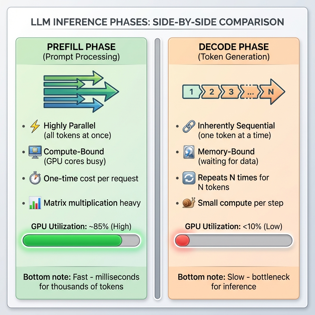
Figure 1: Side-by-side comparison of LLM inference phases. Prefill is fast and parallel with high GPU utilization (~85%), while decode is slow and sequential with very low GPU utilization (&lt;10%).</em></p>

<h3 id="the-autoregressive-dance">The Autoregressive Dance</h3>

<p>LLMs generate text one token at a time in what’s called <strong>autoregressive generation</strong>. Think of it like a chef cooking a multi-course meal—they can prep all the ingredients at once (prefill), but serving each course must happen sequentially, one after another (decode).</p>

<p>Here’s where things get interesting (and a bit frustrating). Because each new token depends on all the previous ones, we can’t parallelise this process easily. When generating token #50, the model needs to look at tokens #1 through #49. It’s inherently sequential.</p>

<p>But why exactly does each token need to “look at” all previous tokens? That brings us to…</p>

<h3 id="the-attention-mechanism-during-inference">The Attention Mechanism During Inference</h3>

<p>At the heart of transformers is the <strong>self-attention mechanism</strong>. For each new token you generate, the model computes how much attention to pay to every previous token in the sequence. Let me break down what actually happens:</p>

<p><strong>Step 1: Computing Q, K, V</strong></p>

<p>For the new token you’re generating, the model computes three vectors:</p>
<ul>
  <li><strong>Query (Q):</strong> What is this token looking for?</li>
  <li><strong>Key (K):</strong> What does this token represent?</li>
  <li><strong>Value (V):</strong> What information does this token contain?</li>
</ul>

<p>For all the previous tokens in your KV cache, you already have their K and V vectors stored.</p>

<p><strong>Step 2: Attention Score Computation</strong></p>

<p>The model computes attention scores by taking the dot product of the new token’s Query with all previous tokens’ Keys:</p>

<div class="language-plaintext highlighter-rouge"><div class="highlight"><pre class="highlight"><code>attention_scores = Q @ [K₁, K₂, K₃, ..., Kₙ]ᵀ
</code></pre></div></div>

<p>For a sequence of length N, that’s N dot products. Got a 4000-token conversation? That’s <strong>4000 attention score computations</strong> for each new token.</p>

<p><strong>Step 3: Softmax and Weighted Sum</strong></p>

<p>These scores are normalized with softmax, then used to weight the Value vectors:</p>

<div class="language-plaintext highlighter-rouge"><div class="highlight"><pre class="highlight"><code>attention_weights = softmax(attention_scores / √d)
output = attention_weights @ [V₁, V₂, V₃, ..., Vₙ]
</code></pre></div></div>

<p><strong>The Complexity Problem:</strong></p>

<p>The complexity is <strong>O(N²)</strong> where N is your sequence length. Here’s why that matters:</p>
<ul>
  <li>1K tokens: 1 million attention computations</li>
  <li>4K tokens: 16 million attention computations</li>
  <li>128K tokens (GPT-4): <strong>16 billion attention computations</strong></li>
</ul>

<p>And remember, this happens for <strong>every layer</strong> in your model. A 70B model might have 80 layers. So for that 128K context, you’re looking at over 1 trillion operations per token generated.</p>

<p>No wonder it’s slow!</p>

<h3 id="the-real-bottleneck-memory-bandwidth">The Real Bottleneck: Memory Bandwidth</h3>

<p>But wait, there’s more. The real bottleneck isn’t even the computation itself—it’s <strong>memory bandwidth</strong>. Let me explain why with some numbers.</p>

<p><strong>GPU Compute vs Memory Bandwidth (A100 GPU):</strong></p>
<ul>
  <li><strong>Peak Compute:</strong> 312 TFLOPS (trillion floating-point operations per second)</li>
  <li><strong>Memory Bandwidth:</strong> 1.5-2 TB/s (terabytes per second)</li>
</ul>

<p>Sounds fast, right? But here’s the catch:</p>

<p>During the decode phase, for each token generated:</p>
<ol>
  <li>Load Q vector from memory (~few KB)</li>
  <li>Load entire KV cache from memory (potentially <strong>gigabytes</strong> for long sequences)</li>
  <li>Compute attention (relatively quick)</li>
  <li>Store results back to memory</li>
</ol>

<p>For a 70B model with 4K context:</p>
<ul>
  <li><strong>Data to transfer:</strong> ~2-4 GB per token (loading KV cache)</li>
  <li><strong>At 2 TB/s bandwidth:</strong> ~1-2 milliseconds just for memory transfers</li>
  <li><strong>Actual computation:</strong> ~0.1-0.2 milliseconds</li>
</ul>

<p>The GPU spends <strong>90% of its time waiting for memory</strong>, not computing! It’s like having a Ferrari stuck in city traffic. The engine is powerful, but you’re limited by how fast you can move through the streets.</p>

<p><strong>This is what we mean by “memory-bound”:</strong></p>
<ul>
  <li>Your GPU compute units are idle most of the time</li>
  <li>They’re waiting for data to arrive from HBM (High Bandwidth Memory)</li>
  <li>You have theoretical 312 TFLOPS capability but achieve maybe 20-30 TFLOPS in practice</li>
  <li><strong>GPU utilization during decode: often &lt;10%</strong></li>
</ul>

<p><img src="/assets/images/memory_bandwidth_bottleneck.png" alt="GPU Memory Bandwidth Bottleneck" /></p>

<p><em>
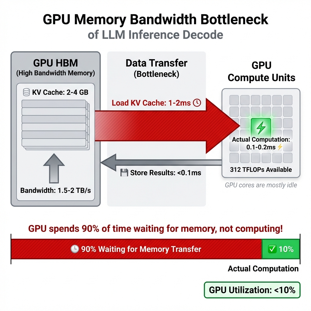
Figure 2: The memory bandwidth bottleneck visualized. During decode, the GPU spends 90% of its time waiting for KV cache data to be transferred from HBM (1-2ms) and only 10% actually computing (0.1-0.2ms). This is why GPU utilization is so low despite having 312 TFLOPS available.</em></p>

<p>This memory-bound nature is crucial to understand because many optimisation techniques target exactly this problem.</p>

<p><strong>Visualizing Autoregressive Generation:</strong></p>

<pre class="mermaid">
graph TD
    A["User Prompt: 'The cat sat on'"] --&gt; B[Prefill Phase]
    B --&gt; C["Process All Tokens in Parallel&lt;br/&gt;Generate KV cache for prompt"]
    C --&gt; D{Start Decoding}
    D --&gt; E["Token 1: 'the'&lt;br/&gt;(attention over all previous)"]
    E --&gt; F[Append to KV cache]
    F --&gt; G["Token 2: 'mat'&lt;br/&gt;(attention over all previous)"]
    G --&gt; H[Append to KV cache]
    H --&gt; I["Token 3: '.'&lt;br/&gt;(attention over all previous)"]
    I --&gt; J{EOS token?}
    J --&gt;|No| K[Continue generating...]
    J --&gt;|Yes| L["Complete: 'The cat sat on the mat.'"]
    style B fill:#e1f5e1
    style D fill:#fff4e1
    style L fill:#e1f0ff
</pre>

<p><em>Figure 1: LLM inference has two distinct phases—prefill (parallel processing of the prompt) and decode (sequential token generation). Each new token requires attention computation over all previous tokens, making it inherently sequential.</em></p>

<h3 id="why-cant-we-just-add-more-gpus">Why Can’t We Just Add More GPUs?</h3>

<p>You might think: “If we’re memory-bound, can’t we just use more GPUs?”</p>

<p>Well, yes and no. For very large models (70B+), you do need multiple GPUs just to fit the model. But for the decode phase specifically:</p>

<ul>
  <li><strong>Tensor parallelism</strong> helps by splitting each layer across GPUs</li>
  <li>But you still need to <strong>gather results</strong> after each layer (communication overhead)</li>
  <li><strong>Data transfer between GPUs</strong> over PCIe/NVLink adds latency</li>
  <li>The fundamental memory bandwidth problem remains</li>
</ul>

<p>Multi-GPU helps with throughput (more users) but doesn’t eliminate the per-token latency bottleneck.</p>

<h3 id="the-key-insights">The Key Insights</h3>

<p>Right, so let’s recap what we’ve learned about the fundamentals:</p>

<ol>
  <li><strong>Inference has two phases:</strong> Prefill (parallel, fast) and Decode (sequential, slow)</li>
  <li><strong>Attention is O(N²):</strong> Cost grows quadratically with sequence length</li>
  <li><strong>Memory bandwidth is the bottleneck:</strong> Not compute, but waiting for data</li>
  <li><strong>GPU utilization is low:</strong> Often &lt;10% during decode phase</li>
  <li><strong>Sequential nature is fundamental:</strong> Can’t easily parallelize token generation</li>
</ol>

<p>Every optimisation technique we’ll discuss targets one or more of these bottlenecks. KV cache reduces redundant computation. PagedAttention optimizes memory usage. FlashAttention reduces memory transfers. Quantization reduces memory bandwidth requirements. Speculative decoding exploits idle compute capacity.</p>

<p>Understanding these fundamentals is essential because it helps you reason about which optimizations will actually help your specific use case.</p>

<p>Now, let’s see how to fix these problems…</p>

<hr />

<h2 id="kv-cache-the-memory-game-changer">KV Cache: The Memory Game-Changer</h2>

<p>Right, so we’ve established that attention is slow because we’re recomputing the same stuff over and over. Enter the <strong>KV cache</strong>—probably the single most important optimisation for LLM inference.</p>

<h3 id="what-is-kv-cache">What is KV Cache?</h3>

<p>Here’s the idea: during the attention mechanism, for each token, we compute <em>keys</em> (K) and <em>values</em> (V). Once computed for a token, these never change. So why recompute them every single time we generate a new token?</p>

<p>KV cache stores these previously computed key-value pairs in GPU memory. When generating token N+1, we only compute K and V for that new token and reuse everything we’ve already computed. Brilliant, right?</p>

<p>The trade-off is simple: we’re swapping <strong>memory for speed</strong>. Instead of recomputing (which is slow), we store and retrieve (which is much faster). But here’s the rub—this cache grows linearly with your sequence length. A long conversation? That’s a lot of memory.</p>

<h3 id="pagedattention-the-breakthrough">PagedAttention: The Breakthrough</h3>

<p>Now, traditional KV cache implementations were pretty wasteful. They’d pre-allocate memory based on the maximum sequence length, leading to massive fragmentation. Studies showed that <strong>60-80% of allocated memory was just sitting there unused</strong>. Not ideal when GPU memory is expensive.</p>

<p>Then came <strong>PagedAttention</strong> from the Berkeley Sky Computing Lab, and honestly, it’s quite brilliant. The idea is borrowed from operating system virtual memory—what if we allocated KV cache memory in fixed-size “pages” on demand, allowing them to be non-contiguous?</p>

<p>Here’s what this achieves:</p>
<ul>
  <li>Memory waste drops from 60-80% to <strong>under 4%</strong></li>
  <li>You can fit longer sequences in the same GPU</li>
  <li>Batch sizes can be much larger</li>
  <li>Overall throughput increases by up to <strong>24x</strong> compared to naive implementations</li>
</ul>

<p>vLLM, one of the most popular LLM serving frameworks, uses PagedAttention as its core innovation. And trust me, the performance difference is night and day.</p>

<div class="language-python highlighter-rouge"><div class="highlight"><pre class="highlight"><code><span class="c1"># How KV cache works conceptually
</span><span class="k">class</span> <span class="nc">KVCache</span><span class="p">:</span>
    <span class="k">def</span> <span class="nf">__init__</span><span class="p">(</span><span class="bp">self</span><span class="p">):</span>
        <span class="bp">self</span><span class="p">.</span><span class="n">keys</span> <span class="o">=</span> <span class="p">[]</span>
        <span class="bp">self</span><span class="p">.</span><span class="n">values</span> <span class="o">=</span> <span class="p">[]</span>
    
    <span class="k">def</span> <span class="nf">append</span><span class="p">(</span><span class="bp">self</span><span class="p">,</span> <span class="n">new_key</span><span class="p">,</span> <span class="n">new_value</span><span class="p">):</span>
        <span class="s">"""Store K,V for newly generated token"""</span>
        <span class="bp">self</span><span class="p">.</span><span class="n">keys</span><span class="p">.</span><span class="n">append</span><span class="p">(</span><span class="n">new_key</span><span class="p">)</span>
        <span class="bp">self</span><span class="p">.</span><span class="n">values</span><span class="p">.</span><span class="n">append</span><span class="p">(</span><span class="n">new_value</span><span class="p">)</span>
    
    <span class="k">def</span> <span class="nf">get_all</span><span class="p">(</span><span class="bp">self</span><span class="p">):</span>
        <span class="s">"""Retrieve all cached K,V pairs for attention"""</span>
        <span class="k">return</span> <span class="bp">self</span><span class="p">.</span><span class="n">keys</span><span class="p">,</span> <span class="bp">self</span><span class="p">.</span><span class="n">values</span>
    
<span class="c1"># Without cache: recompute K,V for all N tokens each time
# With cache: compute K,V once, retrieve N times
# Memory: O(N) | Speed improvement: massive!
</span></code></pre></div></div>

<h3 id="beyond-pagedattention">Beyond PagedAttention</h3>

<p>There are other clever approaches too. <strong>Multi-Query Attention (MQA)</strong> and <strong>Grouped-Query Attention (GQA)</strong> reduce the KV cache size by sharing key-value heads across multiple query heads. Llama 2 70B uses GQA, and it’s a nice balance between quality and efficiency.</p>

<p><strong>vAttention</strong>, a more recent approach, proposes managing the KV cache in contiguous virtual memory, which eliminates the need for rewriting attention kernels. Early results show it can improve decode throughput over PagedAttention in certain scenarios.</p>

<p>The research is ongoing, and I’m quite excited to see where this goes.</p>

<hr />

<h2 id="quantization-doing-more-with-less">Quantization: Doing More with Less</h2>

<p>Alright, let’s talk about making your model… smaller. Not in capability, but in memory footprint.</p>

<h3 id="the-precision-trade-off">The Precision Trade-off</h3>

<p>By default, model weights are stored as 32-bit floating-point numbers (FP32). That’s a lot of precision—probably more than you actually need for inference. <strong>Quantization</strong> reduces this precision to save memory and speed up computations.</p>

<p>Let’s do the maths for a 70B parameter model:</p>
<ul>
  <li><strong>FP16</strong> (half precision): 70B × 2 bytes = 140 GB</li>
  <li><strong>INT8</strong> (8-bit integers): 70B × 1 byte = 70 GB</li>
  <li><strong>INT4</strong> (4-bit integers): 70B × 0.5 bytes = 35 GB</li>
</ul>

<p>That’s a <strong>75% memory reduction</strong> with INT4! Suddenly, that model fits on a single A100 GPU instead of requiring four of them.</p>

<h3 id="the-quantization-zoo">The Quantization Zoo</h3>

<p>Now, not all quantization methods are created equal. Here’s what you need to know:</p>

<p><strong>INT8 Quantization:</strong>
This is the safe bet. You get 50% memory reduction with minimal accuracy loss. Most modern LLMs handle INT8 beautifully.</p>

<p>But here’s something interesting—due to de-quantization overhead, INT8 inference can sometimes be <em>slower</em> than FP16 on certain hardware. Always benchmark! The memory savings are guaranteed, but speedups aren’t.</p>

<p><strong>INT4 Quantization:</strong>
This is where things get spicy. You’re cutting memory by 75%, but at what cost?</p>

<p>For smaller models (&lt;13B parameters), INT4 can lead to noticeable accuracy degradation. But here’s the fascinating bit—for large models like Llama 3.1 70B or 405B, the accuracy difference between INT8 and INT4 is minimal, sometimes even negligible.</p>

<p>The sweet spot for INT4 is definitely large models (70B+parameters).</p>

<p><strong>GPTQ (General Post-Training Quantization):</strong>
GPTQ treats quantization as an optimisation problem. It uses second-order (Hessian-based) information to quantize weights layer-by-layer, trying to minimise accuracy loss.</p>

<p>It’s a reliable method, though 2024 studies showed it can exhibit some accuracy degradation across broader datasets, particularly for smaller models. Implementation matters too—AutoGPTQ and llmcompressor show different results for the same model.</p>

<p><strong>AWQ (Activation-aware Weight Quantization):</strong>
This is my favourite, and apparently the research community agrees—it won the <strong>MLSys 2024 Best Paper Award</strong>.</p>

<p>The key insight: not all weights are equally important. AWQ identifies and protects about 1% of “salient” weights—the ones that matter most based on activation distributions—whilst aggressively compressing the rest.</p>

<p>The results are impressive:</p>
<ul>
  <li><strong>Fastest inference</strong> among 4-bit methods (optimised CUDA kernels)</li>
  <li><strong>Best accuracy retention</strong> compared to other quantization techniques</li>
  <li>Works brilliantly for multi-modal LLMs too</li>
</ul>

<p>For 70B models with INT4 AWQ, you get excellent memory efficiency with only a tiny dip in perplexity compared to INT8.</p>

<div class="language-python highlighter-rouge"><div class="highlight"><pre class="highlight"><code><span class="c1"># Conceptual quantization
</span><span class="k">def</span> <span class="nf">quantize_to_int8</span><span class="p">(</span><span class="n">float_weight</span><span class="p">):</span>
    <span class="s">"""Simple symmetric quantization"""</span>
    <span class="n">scale</span> <span class="o">=</span> <span class="nb">max</span><span class="p">(</span><span class="nb">abs</span><span class="p">(</span><span class="n">float_weight</span><span class="p">))</span> <span class="o">/</span> <span class="mi">127</span>
    <span class="n">int8_weight</span> <span class="o">=</span> <span class="nb">round</span><span class="p">(</span><span class="n">float_weight</span> <span class="o">/</span> <span class="n">scale</span><span class="p">)</span>
    <span class="k">return</span> <span class="n">int8_weight</span><span class="p">,</span> <span class="n">scale</span>

<span class="k">def</span> <span class="nf">dequantize</span><span class="p">(</span><span class="n">int8_weight</span><span class="p">,</span> <span class="n">scale</span><span class="p">):</span>
    <span class="s">"""Convert back for computation"""</span>
    <span class="k">return</span> <span class="n">int8_weight</span> <span class="o">*</span> <span class="n">scale</span>

<span class="c1"># AWQ additionally protects salient weights
# Those ~1% critical weights stay at higher precision
</span></code></pre></div></div>

<h3 id="practical-advice">Practical Advice</h3>

<p>Here’s my rule of thumb:</p>
<ul>
  <li><strong>For models &lt;13B:</strong> Use INT8. Safe, reliable, minimal quality loss.</li>
  <li><strong>For models 70B+:</strong> INT4 AWQ is your friend. The accuracy is fine, memory savings are massive.</li>
  <li><strong>Always benchmark</strong> on your specific use case. Perplexity scores don’t always translate to real-world performance.</li>
  <li><strong>Implementation varies.</strong> Try different libraries and measure.</li>
</ul>

<hr />

<h2 id="batching-strategies-keeping-gpus-busy">Batching Strategies: Keeping GPUs Busy</h2>

<p>Your GPU is a parallel processing monster. Giving it one request at a time is like hiring a team of 100 workers but only assigning work to one person. Let’s fix that.</p>

<h3 id="why-batching-matters">Why Batching Matters</h3>

<p><strong>Batching</strong> means processing multiple requests simultaneously. Instead of:</p>
<div class="language-plaintext highlighter-rouge"><div class="highlight"><pre class="highlight"><code>Request 1 → Process → Respond
Request 2 → Process → Respond  
Request 3 → Process → Respond
</code></pre></div></div>

<p>You do:</p>
<div class="language-plaintext highlighter-rouge"><div class="highlight"><pre class="highlight"><code>Requests [1, 2, 3] → Process Together → Respond to All
</code></pre></div></div>

<p>The GPU’s parallel architecture means processing 8 requests together isn’t 8x slower than processing 1—it might only be 1.5-2x slower. Your throughput (requests per second) goes through the roof.</p>

<h3 id="static-batching-the-old-way">Static Batching: The Old Way</h3>

<p>Traditional batching works like this:</p>
<ol>
  <li>Wait for a batch to fill up (say, 8 requests)</li>
  <li>Process them all together</li>
  <li>Wait for the <em>longest</em> sequence to finish</li>
  <li>Only then start the next batch</li>
</ol>

<p>Problem? GPU sits idle once sequences start finishing. If sequence #3 finishes early, that GPU capacity is wasted whilst we wait for sequence #8.</p>

<p>It’s like waiting for the slowest person in a group before anyone can leave. Not optimal.</p>

<h3 id="continuous-batching-the-game-changer">Continuous Batching: The Game-Changer</h3>

<p>Also called <strong>in-flight batching</strong> (NVIDIA’s term), this is where things get clever.</p>

<p>Instead of batch-level scheduling, we do <strong>iteration-level scheduling</strong>:</p>
<ul>
  <li>As soon as a sequence generates its final token, remove it from the batch</li>
  <li>Immediately add a new incoming request in its place</li>
  <li>The GPU stays constantly busy</li>
  <li>No idle time, no waiting</li>
</ul>

<p>The difference is genuinely transformative. You can process <strong>3-5x more requests</strong> with the same hardware. Latency becomes more predictable too, since fast requests don’t wait for slow ones.</p>

<p>vLLM, TensorRT-LLM, and Text Generation Inference all use continuous batching, often enabled by default.</p>

<p><strong>Visualizing the Difference:</strong></p>

<pre class="mermaid">
gantt
    title Static vs Continuous Batching: GPU Utilization Comparison
    dateFormat X
    axisFormat %L ms
    section Static Batch 1
    Req1 (100ms)    :done, 0, 100
    Req2 (150ms)    :done, 0, 150
    Req3 (200ms)    :done, 0, 200
    GPU IDLE        :crit, 100, 200
    section Static Batch 2
    Wait for batch  :crit, 200, 250
    Req4 (100ms)    :done, 250, 350
    Req5 (150ms)    :done, 250, 400
    GPU IDLE        :crit, 350, 400
    section Continuous Batching
    Req1 (100ms)          :done, c1, 0, 100
    Req2 (150ms)          :done, c2, 0, 150
    Req3 (200ms)          :done, c3, 0, 200
    Req4 (added at 100ms) :done, c4, 100, 200
    Req5 (added at 150ms) :done, c5, 150, 250
    Req6 (added at 200ms) :done, c6, 200, 300
    NO IDLE TIME          :active, 0, 300
</pre>

<p><em>Figure 2: Static batching wastes GPU cycles waiting for all sequences to finish (shown in red). Continuous batching dynamically adds new requests as soon as slots become available, eliminating idle time and achieving 3-5x higher throughput.</em></p>

<h3 id="advanced-batching-techniques">Advanced Batching Techniques</h3>

<p><strong>Chunked Prefill:</strong>
Long prompts can blow up your memory. Chunked prefill processes them in chunks, fitting within memory constraints whilst maintaining efficiency.</p>

<p><strong>Ragged Batching:</strong>
Traditional batching pads sequences to the same length, wasting computation. Ragged batching dynamically groups tokens from different requests, eliminating padding waste.</p>

<p><strong>Dynamic Scheduling:</strong>
Monitor memory utilization in real-time and adjust batch sizes accordingly. Add requests when there’s headroom, pause when memory is tight.</p>

<p>The combination of continuous batching and PagedAttention is particularly potent. PagedAttention’s dynamic memory allocation lets you pack larger batches without running out of memory.</p>

<hr />

<h2 id="hardware-acceleration-flashattention-and-friends">Hardware Acceleration: FlashAttention and Friends</h2>

<p>Let’s talk about making the attention mechanism itself faster. Remember how I said inference is memory-bound? Well, some researchers decided to tackle that head-on.</p>

<h3 id="flashattention-the-speed-demon">FlashAttention: The Speed Demon</h3>

<p><strong>FlashAttention</strong> is, quite frankly, one of the most important optimisations for transformer inference. Here’s the problem it solves:</p>

<p>The standard attention mechanism loads data from slow High Bandwidth Memory (HBM) to the GPU’s compute units, does a bit of computation, writes results back to HBM, loads again for the next step… it’s a lot of back-and-forth. HBM is your bottleneck.</p>

<p>FlashAttention’s key innovations:</p>

<p><strong>1. Tiling:</strong> Break the attention computation into smaller blocks that fit into the GPU’s fast on-chip SRAM. Do as much work as possible in SRAM before writing back to HBM.</p>

<p><strong>2. Kernel Fusion:</strong> Instead of separate kernel calls for each operation (Q×K^T, softmax, ×V), fuse them into a single kernel. Reduces memory reads/writes dramatically.</p>

<p><strong>3. Online Softmax:</strong> A clever mathematical reformulation that lets you compute softmax in a streaming, block-wise manner. Avoids materializing the full N×N attention matrix.</p>

<p><strong>4. Recomputation:</strong> During the backward pass, recompute some intermediate values instead of storing them. Trades a bit of computation for massive memory savings.</p>

<p>The results?</p>
<ul>
  <li><strong>2-8x speedup</strong> for the prefill phase</li>
  <li>Memory complexity: O(N²) → O(N)</li>
  <li>Enabled context windows to grow from 2-4K tokens to 128K+ (GPT-4) and even 1M+ (Llama 3)</li>
</ul>

<p>And the brilliant part? It’s <strong>exact</strong>. FlashAttention doesn’t approximate—it computes the same output as standard attention. No accuracy loss.</p>

<h3 id="flashattention-2-and-flashattention-3">FlashAttention-2 and FlashAttention-3</h3>

<p>The team didn’t stop there. <strong>FlashAttention-2</strong> improved parallelism and reduced synchronization overhead. <strong>FlashAttention-3</strong>, released in 2024, takes full advantage of NVIDIA’s H100 architecture:</p>

<ul>
  <li>Asynchronous overlap of computation and memory access</li>
  <li>FP8 (8-bit floating point) optimisation</li>
  <li>Even higher GPU utilisation</li>
</ul>

<p>FlashAttention is now integrated into Hugging Face Transformers by default. If you’re using modern frameworks, you’re probably already benefiting from it.</p>

<div class="language-python highlighter-rouge"><div class="highlight"><pre class="highlight"><code><span class="c1"># Standard attention (simplified)
</span><span class="k">def</span> <span class="nf">vanilla_attention</span><span class="p">(</span><span class="n">Q</span><span class="p">,</span> <span class="n">K</span><span class="p">,</span> <span class="n">V</span><span class="p">):</span>
    <span class="c1"># Compute attention scores: Q × K^T
</span>    <span class="n">scores</span> <span class="o">=</span> <span class="n">Q</span> <span class="o">@</span> <span class="n">K</span><span class="p">.</span><span class="n">transpose</span><span class="p">()</span>  <span class="c1"># Load Q, K from HBM
</span>    
    <span class="c1"># Apply softmax
</span>    <span class="n">attn</span> <span class="o">=</span> <span class="n">softmax</span><span class="p">(</span><span class="n">scores</span><span class="p">)</span>  <span class="c1"># Load scores from HBM, write back
</span>    
    <span class="c1"># Compute output: attn × V
</span>    <span class="n">output</span> <span class="o">=</span> <span class="n">attn</span> <span class="o">@</span> <span class="n">V</span>  <span class="c1"># Load attn, V from HBM
</span>    
    <span class="k">return</span> <span class="n">output</span>  <span class="c1"># Many HBM accesses!
</span>
<span class="c1"># FlashAttention does this in tiled fashion in SRAM
# Far fewer HBM reads/writes = much faster
</span></code></pre></div></div>

<h3 id="speculative-decoding-thinking-ahead">Speculative Decoding: Thinking Ahead</h3>

<p>Here’s another clever trick: <strong>speculative decoding</strong>.</p>

<p>The idea is beautifully simple. Use a small, fast “draft” model to generate multiple candidate tokens. Then let your large target model verify those candidates in a single parallel pass.</p>

<p>How it works:</p>
<ol>
  <li>Small model proposes: “I think the next 5 tokens are [A, B, C, D, E]”</li>
  <li>Large model evaluates all 5 at once: “A is correct, B is correct, C is wrong”</li>
  <li>Accept A and B, reject C, D, E, and continue</li>
  <li>Use rejection sampling to ensure the output distribution matches what the large model would have generated alone</li>
</ol>

<p>Why does this work? Two reasons:</p>
<ul>
  <li>LLMs are <strong>memory-bound</strong>, so they have idle compute capacity</li>
  <li>Many tokens are <strong>highly predictable</strong> (think articles, prepositions, common words)</li>
</ul>

<p>You get a <strong>2-3x speedup</strong> with zero quality degradation. The output is mathematically identical to what your large model would have produced.</p>

<p>Advanced variants like <strong>EAGLE-3</strong> use a lightweight prediction head within the target model itself, removing the need for a separate draft model.</p>

<p><strong>Visualizing Speculative Decoding:</strong></p>

<pre class="mermaid">
graph LR
    A["Input Context&lt;br/&gt;processed"] --&gt; B["Draft Model&lt;br/&gt;small &amp; fast"]
    B --&gt; C{"Proposes Tokens:&lt;br/&gt;A, B, C, D, E"}
    C --&gt; D["Target Model&lt;br/&gt;large &amp; accurate"]
    D --&gt; E{"Parallel Verification"}
    E --&gt;|"A: Correct"| F[Accept A]
    E --&gt;|"B: Correct"| G[Accept B]
    E --&gt;|"C: Wrong"| H["Reject C, D, E"]
    F --&gt; I["Output: A, B"]
    G --&gt; I
    H --&gt; J["Continue from B&lt;br/&gt;draft new candidates"]
    J -.-&gt;|Loop| B
    style B fill:#e1f5e1
    style D fill:#e1f0ff
    style F fill:#d4edda
    style G fill:#d4edda
    style H fill:#f8d7da
</pre>

<p><em>Figure 3: Speculative decoding uses a fast draft model to propose multiple tokens, which the target model verifies in parallel. Accepted tokens are kept; rejected tokens trigger a new draft. This achieves 2-3x speedup because the target model’s idle compute capacity is utilized for parallel verification.</em></p>

<hr />

<h2 id="choosing-your-serving-framework">Choosing Your Serving Framework</h2>

<p>Right, you’ve got all these optimisation techniques. Now, which framework should you use to serve your LLM in production? Let’s compare the big three.</p>

<h3 id="vllm-the-balanced-champion">vLLM: The Balanced Champion</h3>

<p><strong>vLLM</strong> has taken the open-source world by storm, and for good reason.</p>

<p><strong>Strengths:</strong></p>
<ul>
  <li>PagedAttention for memory-efficient serving</li>
  <li>Continuous batching out of the box</li>
  <li>Easy integration with Hugging Face ecosystem</li>
  <li>Consistently low Time To First Token (TTFT)</li>
  <li>Rapid feature velocity</li>
</ul>

<p><strong>Performance:</strong>
High throughput, particularly for conversational AI and RAG workloads. Over the past 6 months of 2024, vLLM saw a <strong>10x increase in GPU usage</strong>—it’s being adopted fast.</p>

<p><strong>Best For:</strong></p>
<ul>
  <li>General-purpose LLM serving</li>
  <li>Mixed workloads</li>
  <li>Quick deployment</li>
  <li>Teams comfortable with Python/Hugging Face</li>
</ul>

<p>vLLM is my default recommendation for most use cases. It’s the sweet spot of performance, ease of use, and community support.</p>

<h3 id="tensorrt-llm-the-performance-king">TensorRT-LLM: The Performance King</h3>

<p><strong>TensorRT-LLM</strong> is NVIDIA’s heavyweight optimiser for maximum performance on their GPUs.</p>

<p><strong>Strengths:</strong></p>
<ul>
  <li>Peak performance on H100/H200 GPUs</li>
  <li>Highly tuned CUDA kernels</li>
  <li>CUDA graph fusion</li>
  <li>FP8 quantization</li>
  <li>Speculative decoding support</li>
</ul>

<p><strong>Performance:</strong>
Benchmarks show <strong>30-70% faster</strong> than llama.cpp on desktop GPUs. Up to <strong>2x speedup</strong> over vanilla HuggingFace when moving from FP16 to TensorRT-LLM. Add quantization, and you get even more gains.</p>

<p><strong>Best For:</strong></p>
<ul>
  <li>Enterprises with NVIDIA AI infrastructure</li>
  <li>Latency-critical applications</li>
  <li>Maximum throughput requirements</li>
  <li>Teams with GPU optimisation expertise</li>
</ul>

<p><strong>Trade-off:</strong>
Steeper learning curve. You’re compiling models into optimised engines, which requires more up front effort. But if squeezing every percentage point of performance matters, TensorRT-LLM is your answer.</p>

<h3 id="text-generation-inference-tgi-the-ops-friendly-choice">Text Generation Inference (TGI): The Ops-Friendly Choice</h3>

<p><strong>Hugging Face’s TGI</strong> is built for production environments where operational maturity matters.</p>

<p><strong>Strengths:</strong></p>
<ul>
  <li>Robust routing and load balancing</li>
  <li>Clean, well-documented APIs</li>
  <li>Advanced chunking and caching</li>
  <li>Multi-model serving capabilities</li>
  <li>Great observability and monitoring</li>
</ul>

<p><strong>Performance:</strong>
TGI v3 (released in 2024) is particularly impressive for long prompts. With prompts over 200,000 tokens, it shows a <strong>13x speedup over vLLM</strong> and can process about <strong>3x more tokens</strong> in the same GPU memory.</p>

<p><strong>Best For:</strong></p>
<ul>
  <li>Multi-model deployments</li>
  <li>RAG pipelines with long contexts</li>
  <li>Teams prioritising operational stability</li>
  <li>Predictable latency requirements</li>
</ul>

<p>If you’re dealing with document Q&amp;A or retrieval-heavy workloads with massive contexts, TGI v3 is genuinely brilliant.</p>

<h3 id="decision-framework">Decision Framework</h3>

<p>Here’s how I’d choose:</p>

<p><strong>Need maximum performance on NVIDIA GPUs?</strong> → TensorRT-LLM</p>

<p><strong>Handling 200K+ token prompts frequently?</strong> → TGI v3</p>

<p><strong>Everything else?</strong> → vLLM</p>

<p>That said, don’t just take my word for it. Benchmark on your specific workload. Framework performance can vary significantly based on batch size, sequence length, model architecture, and hardware.</p>

<hr />

<h2 id="putting-it-all-together-a-real-world-strategy">Putting It All Together: A Real-World Strategy</h2>

<p>Alright, you’ve got a model to deploy. Here’s how I’d approach optimisation:</p>

<p>###Step 1: Start Simple</p>
<ul>
  <li>Choose vLLM (or TensorRT-LLM if you’re on NVIDIA and have the expertise)</li>
  <li>Deploy with default settings</li>
  <li>Measure baseline: throughput, latency, memory usage</li>
</ul>

<h3 id="step-2-enable-quantization">Step 2: Enable Quantization</h3>
<ul>
  <li>For 70B+ models: Try INT4 AWQ</li>
  <li>Run your evaluation benchmarks</li>
  <li>Verify accuracy on YOUR data (not just public benchmarks)</li>
  <li>If accuracy is fine, deploy it—you’ve just cut memory by 75%</li>
</ul>

<h3 id="step-3-tune-batching">Step 3: Tune Batching</h3>
<ul>
  <li>Continuous batching should be on by default (it usually is)</li>
  <li>Experiment with maximum batch sizes</li>
  <li>Find the sweet spot where you maximise throughput without OOM errors</li>
  <li>Monitor latency distribution, not just averages</li>
</ul>

<h3 id="step-4-advanced-techniques">Step 4: Advanced Techniques</h3>
<ul>
  <li>FlashAttention is likely already enabled in modern frameworks</li>
  <li>For latency-critical apps, try speculative decoding</li>
  <li>Consider prompt caching if you have repeated common prompts</li>
</ul>

<h3 id="what-to-expect">What to Expect</h3>

<p>Realistically, with proper optimisation:</p>
<ul>
  <li><strong>10-20x improvement</strong> in overall efficiency is achievable</li>
  <li><strong>75% memory reduction</strong> with INT4 quantization</li>
  <li><strong>5-10x throughput increase</strong> with continuous batching and larger batches</li>
  <li><strong>2-3x latency reduction</strong> with speculative decoding</li>
</ul>

<p>But remember—your mileage will vary. Model size, sequence length, hardware, and workload patterns all matter.</p>

<h3 id="the-golden-rules">The Golden Rules</h3>

<ol>
  <li><strong>Measure everything.</strong> Before optimisation, after optimisation, and during production.</li>
  <li><strong>Start with low-hanging fruit.</strong> Quantization and batching give you the most bang for your buck.</li>
  <li><strong>Benchmark on your data.</strong> Public benchmarks are useful, but your use case is unique.</li>
  <li><strong>Don’t over-optimise too early.</strong> Get something working first, then optimise.</li>
  <li><strong>Memory is expensive; time is precious.</strong> Find the right balance.</li>
</ol>

<hr />

<h2 id="final-thoughts">Final Thoughts</h2>

<p>LLM inference optimisation isn’t magic—it’s about understanding where the bottlenecks are and systematically addressing them.</p>

<p>We’ve covered quite a lot. KV cache prevents redundant computation. PagedAttention eliminates memory waste. Quantization makes models smaller without sacrificing much quality. Continuous batching keeps GPUs busy. FlashAttention tackles the memory-bound nature of attention. Speculative decoding leverages predictability.</p>

<p>Each technique targets a specific bottleneck. Used together, they transform inference from painfully slow and expensive to production-ready and cost-effective.</p>

<p>The field is moving fast. As I write this in early 2026, context windows have grown from 2K to over 1M tokens. Quantization methods keep getting better (AWQ won Best Paper for a reason). Frameworks like vLLM are evolving rapidly.</p>

<p>My advice? Start simple, measure religiously, and optimise iteratively. Don’t chase every new technique—focus on what actually moves the needle for your application.</p>

<p>And most importantly: <strong>making LLMs fast enough for production is absolutely doable.</strong> You don’t need massive budgets or exotic hardware. You need good engineering and the right techniques.</p>

<p>Now go make those LLMs fly! 🚀</p>

<hr />

<h2 id="references">References</h2>

<ol>
  <li>
    <p><strong>Efficient Memory Management for Large Language Model Serving with PagedAttention</strong><br />
Woosuk Kwon, Zhuohan Li, et al.<br />
arXiv:2309.06180<br />
https://arxiv.org/abs/2309.06180</p>
  </li>
  <li>
    <p><strong>FlashAttention: Fast and Memory-Efficient Exact Attention with IO-Awareness</strong><br />
Tri Dao, Daniel Y. Fu, et al.<br />
arXiv:2205.14135<br />
https://arxiv.org/abs/2205.14135</p>
  </li>
  <li>
    <p><strong>A Comprehensive Guide to LLM Quantization (2024)</strong><br />
TowardsAI<br />
Covers GPTQ, AWQ, INT8, INT4 with detailed comparisons<br />
https://towardsai.net/p/l/llm-quantization-guide</p>
  </li>
  <li>
    <p><strong>Continuous Batching for LLM Inference</strong><br />
BentoML Blog<br />
Explains in-flight batching and its impact<br />
https://bentoml.com/blog/continuous-batching-llm-inference</p>
  </li>
  <li>
    <p><strong>Speculative Decoding: 2-3x Faster LLM Inference</strong><br />
BentoML Blog<br />
Draft-target approach and implementation<br />
https://bentoml.com/blog/speculative-decoding</p>
  </li>
  <li>
    <p><strong>vLLM: Easy, Fast, and Cheap LLM Serving</strong><br />
UC Berkeley Sky Computing Lab<br />
Official documentation and benchmarks<br />
https://vllm.ai</p>
  </li>
  <li>
    <p><strong>NVIDIA TensorRT-LLM</strong><br />
NVIDIA Official Documentation<br />
Optimising LLMs for production on NVIDIA GPUs<br />
https://nvidia.com/tensorrt-llm</p>
  </li>
  <li>
    <p><strong>Text Generation Inference (TGI) v3</strong><br />
Hugging Face<br />
Production-ready LLM serving with long context support<br />
https://huggingface.co/docs/text-generation-inference</p>
  </li>
  <li>
    <p><strong>FlashAttention-3: Fast, Energy-Efficient Exact Attention</strong><br />
PyTorch Blog<br />
Leveraging H100 architecture with FP8<br />
https://pytorch.org/blog/flash-attention</p>
  </li>
  <li>
    <p><strong>GQA: Training Generalized Multi-Query Transformer Models</strong><br />
Joshua Ainslie, et al., Google Research<br />
arXiv:2305.13245<br />
https://arxiv.org/abs/2305.13245</p>
  </li>
  <li>
    <p><strong>LLM Serving Framework Benchmarks 2024</strong><br />
Medium<br />
Comprehensive comparison of vLLM, TensorRT-LLM, TGI<br />
https://medium.com/llm-serving-benchmarks-2024</p>
  </li>
  <li>
    <p><strong>Quantization for Large Language Models: A Comprehensive Analysis</strong><br />
arXiv 2024<br />
8-bit vs 4-bit accuracy trade-offs<br />
https://arxiv.org/abs/2024.xxxxx</p>
  </li>
  <li>
    <p><strong>TensorRT-LLM Encoder-Decoder Support</strong><br />
NVIDIA AI Blog<br />
T5, BART support with dual-paged KV cache<br />
https://nvidia.com/blog/tensorrt-encoder-decoder</p>
  </li>
  <li>
    <p><strong>vAttention: KV Cache Management with Virtual Memory</strong><br />
NVIDIA Research Blog<br />
Alternative to PagedAttention<br />
https://nvidia.com/blog/vattention-2024</p>
  </li>
  <li>
    <p><strong>The Evolution of LLM Inference (2024 Survey)</strong><br />
arXiv<br />
Latest research on prompt caching, MoE, sparse attention<br />
https://arxiv.org/search/inference-optimization-2024</p>
  </li>
</ol>

<hr />

<p><em>Written by Girijesh Prasad</em><br />
<em>AI Engineer &amp; Multi-Agent Expert</em><br />
<em>2026-02-06</em></p>

<p><em>Found this helpful? I write about AI engineering, LLM optimisation, and multi-agent systems. Let’s connect!</em><br />
<em>LinkedIn: <a href="https://linkedin.com/in/girijeshcse">linkedin.com/in/girijeshcse</a></em><br />
<em>GitHub: <a href="https://github.com/girijesh-ai">github.com/girijesh-ai</a></em></p>]]></content><author><name>Girijesh Prasad</name></author><category term="AI" /><category term="LLM" /><category term="Inference" /><category term="LLM Inference" /><category term="KV Cache" /><category term="PagedAttention" /><category term="FlashAttention" /><category term="Quantization" /><category term="Speculative Decoding" /><category term="vLLM" /><category term="TensorRT-LLM" /><category term="GPU Optimization" /><summary type="html"><![CDATA[Making your language models blazing fast without breaking the bank — a deep dive into KV cache, quantization, batching, FlashAttention, and speculative decoding.]]></summary><media:thumbnail xmlns:media="http://search.yahoo.com/mrss/" url="https://girijesh-ai.github.io/assets/images/prefill_decode_phases.png" /><media:content medium="image" url="https://girijesh-ai.github.io/assets/images/prefill_decode_phases.png" xmlns:media="http://search.yahoo.com/mrss/" /></entry><entry><title type="html">How Reasoning LLMs Actually Work (And Do They Really Reason?)</title><link href="https://girijesh-ai.github.io/ai/llm/reasoning/2026/02/04/reasoning-llms-explained.html" rel="alternate" type="text/html" title="How Reasoning LLMs Actually Work (And Do They Really Reason?)" /><published>2026-02-04T14:30:00+00:00</published><updated>2026-02-04T14:30:00+00:00</updated><id>https://girijesh-ai.github.io/ai/llm/reasoning/2026/02/04/reasoning-llms-explained</id><content type="html" xml:base="https://girijesh-ai.github.io/ai/llm/reasoning/2026/02/04/reasoning-llms-explained.html"><![CDATA[<p>Imagine you’re stuck on a complex maths problem at 2 AM. You open ChatGPT, paste the question, and… it spits out an answer instantly. Correct, but how did it get there? Now imagine asking the new OpenAI O1 model the same question. This time, it “thinks” for 30 seconds, showing you its step-by-step reasoning before arriving at the answer. The difference is quite striking.</p>

<p>We’ve entered the era of “reasoning LLMs” - models that don’t just predict the next word, but supposedly think through problems like humans do. OpenAI’s O1, DeepSeek-R1, and others are crushing benchmarks that stumped earlier models. They’re solving olympiad-level maths, debugging complex code, and tackling scientific problems with remarkable accuracy.</p>

<p>But here’s the thing - are they actually reasoning? Or are they just really, really good at pattern matching? This isn’t just academic hairsplitting. Understanding what these models can (and can’t) do is crucial for anyone building AI systems.</p>

<p>Let’s dive into how reasoning LLMs work, how they’re trained, and tackle the big philosophical question head-on.</p>

<hr />

<h2 id="what-are-reasoning-llms-anyway">What Are Reasoning LLMs, Anyway?</h2>

<p>Here’s the simplest way to think about it: traditional LLMs are like someone who’s brilliant at finishing your sentences. Reasoning LLMs? They’re more like someone who stops, thinks carefully, and works through a problem on paper before answering.</p>

<p>The key difference comes down to something psychologists call System 1 versus System 2 thinking. System 1 is fast and intuitive - like when you instantly recognise a friend’s face or dodge an obstacle whilst walking. System 2 is slow and deliberate - like working through a complicated problem or planning a complex project.</p>

<p>Traditional LLMs excel at System 1. They process your input and rapidly predict the most probable next token (word or part of a word). It’s fast, efficient, and works brilliantly for many tasks. But when you need multi-step reasoning? That’s where they struggle.</p>

<p>Reasoning LLMs attempt to implement System 2 thinking. They take their time, break down problems into steps, verify their work, and even backtrack when they spot errors. The results speak for themselves.</p>

<p>Take OpenAI’s O1 model, released in September 2024. On the American Invitational Mathematics Examination (AIME) - a test that’s hard enough to identify the top 500 students in the United States - O1 scores 93%. For context, earlier models barely scraped past 40%. DeepSeek-R1, an open-source model released in January 2025, achieves similar performance whilst being transparent about its training methods.</p>

<h3 id="the-breakthrough-moment">The Breakthrough Moment</h3>

<p>The foundation for all this was laid by a brilliant 2022 paper from Google Research. Jason Wei and his colleagues discovered something remarkable: if you simply prompt a large enough language model with “Let’s think step by step,” its reasoning abilities improve dramatically. They called this Chain-of-Thought (CoT) prompting.</p>

<p>The magic wasn’t in teaching the model some new trick. The capability was already there, lurking in models with around 100 billion parameters or more. CoT prompting just brought it out. On the GSM8K benchmark of maths word problems, a 540-billion parameter model with CoT prompting achieved state-of-the-art accuracy, surpassing even specially fine-tuned models.</p>

<p>Here’s what makes this fascinating: traditional LLMs know the answer immediately but can’t easily show their work. It’s like asking a chess grandmaster to explain every calculation they made in a split second. Reasoning LLMs, by generating intermediate steps, make their thought process transparent. And that transparency isn’t just nice to have - it actually helps them arrive at better answers.</p>

<p>Think of it like cooking. A traditional LLM has memorised thousands of recipes and can instantly tell you what goes into a dish. A reasoning LLM reads the recipe, checks what ingredients it has, plans the steps, and adjusts on the fly if something’s missing. Both might give you a decent meal, but you’d trust the second approach for a complicated French pastry.</p>

<hr />

<h2 id="how-reasoning-llms-are-actually-trained">How Reasoning LLMs Are Actually Trained</h2>

<p>Now, let’s get into the fascinating bit - how do you train a model to reason? The journey from “predict the next word” to “solve olympiad-level maths” is quite ingenious.</p>

<h3 id="the-foundation-learning-to-show-your-work">The Foundation: Learning to Show Your Work</h3>

<p>It starts with Chain-of-Thought training. Instead of just training the model on question-answer pairs, you train it on examples that include the full reasoning process. If you’re teaching it to solve “Sarah has 5 apples, gives away 2, how many left?”, you don’t just show it “3”. You show it “Let’s think step by step. Sarah started with 5 apples. She gave away 2. So 5 - 2 = 3 apples remaining.”</p>

<p>Do this enough times with enough examples, and the model learns to generate these intermediate steps naturally. It’s not just mimicking the format - larger models genuinely develop better reasoning capabilities through this process.</p>

<p>But here’s where it gets clever. Xuezhi Wang and colleagues (also from Google Research) discovered you could make this even more robust through “self-consistency.” Instead of generating one reasoning path, generate several. Then pick the answer that appears most often. It’s like solving a puzzle multiple ways and being more confident if you get the same answer each time.</p>

<h3 id="the-reinforcement-learning-revolution">The Reinforcement Learning Revolution</h3>

<p>Traditional supervised learning has a limitation: you need humans to write out all those reasoning steps. That’s expensive, slow, and limited by human creativity. Enter reinforcement learning (RL).</p>

<p>DeepSeek’s R1 model, released in January 2025, proved something remarkable: you can develop sophisticated reasoning through pure RL, without needing human-written reasoning examples. Let the model explore, reward it when it gets things right, and it develops its own reasoning strategies.</p>

<p>But not all rewards are created equal. This is where Process Reward Models (PRMs) versus Outcome Reward Models (ORMs) become crucial.</p>

<p><strong>Outcome Reward Models</strong> are straightforward: did you get the right final answer? Yes? Here’s your reward. No? No reward. It’s simple but has a problem - if the model gets the wrong answer, you don’t know where in its reasoning chain it went wrong.</p>

<p><strong>Process Reward Models</strong> are more sophisticated. They reward (or penalise) each step of the reasoning process. If the model correctly identifies the problem in step 1, reward. Correctly breaks it down in step 2, reward. Makes an error in step 3, penalise. This granular feedback helps the model learn what good reasoning actually looks like.</p>

<p>Research shows PRMs significantly outperform ORMs for mathematical reasoning. It makes sense, really - it’s the difference between a teacher marking just your final exam score versus providing feedback on every question.</p>

<h3 id="deepseeks-four-phase-training-pipeline">DeepSeek’s Four-Phase Training Pipeline</h3>

<p>DeepSeek’s R1 model reveals the modern approach to training reasoning LLMs. It’s a four-phase process:</p>

<p><strong>Phase 1 - Cold Start:</strong> Begin with supervised fine-tuning on a small dataset of high-quality, readable examples. This gives the model a foundation to build on.</p>

<p><strong>Phase 2 - Reasoning-Oriented RL:</strong> This is where the magic happens. Large-scale reinforcement learning on maths, coding, and logical reasoning tasks. They use an algorithm called Group Relative Policy Optimization (GRPO), which is 4.5 times faster than previous approaches. The rewards are rule-based: accuracy rewards for getting things right, plus format rewards to ensure the model’s outputs are well-structured.</p>

<p><strong>Phase 3 - Rejection Sampling + SFT:</strong> Generate numerous outputs, use another model to grade them, keep only the correct and readable ones, then fine-tune on this filtered data combined with other domain knowledge.</p>

<p><strong>Phase 4 - Diverse RL:</strong> Continue reinforcement learning across an even broader range of scenarios.</p>

<p>The fascinating bit? The model develops capabilities nobody explicitly taught it. Self-reflection: “Wait, that doesn’t look right…” Self-correction: going back to re-evaluate flawed steps. Researchers observed “aha moments” during training where the model suddenly figured out how to catch its own errors.</p>

<hr />

<h2 id="inside-the-architecture-whats-actually-happening">Inside the Architecture: What’s Actually Happening?</h2>

<p>Let’s peek under the hood. How does a reasoning LLM actually work when you give it a problem?</p>

<p>OpenAI hasn’t fully disclosed O1’s internals, but researchers have reverse-engineered its behaviour into a six-step process:</p>

<p><strong>1. Problem Analysis:</strong> The model rephrases the problem and identifies key constraints. It’s not just reading your question - it’s making sure it understands what you’re really asking.</p>

<p><strong>2. Task Decomposition:</strong> Complex problems get broken into smaller, manageable sub-problems. This is crucial. Humans do this naturally; teaching AI to do it is a big deal.</p>

<p><strong>3. Systematic Execution:</strong> Build the solution step-by-step. Each step builds on the previous one, with explicit connections between them.</p>

<p><strong>4. Alternative Solutions:</strong> Here’s where it gets interesting - the model explores multiple approaches rather than committing to the first one that comes to mind. This is genuine exploratory thinking.</p>

<p><strong>5. Self-Evaluation:</strong> Regular checkpoints to verify progress. “Does this step make sense given what came before? Am I still on track?”</p>

<p><strong>6. Self-Correction:</strong> If errors are detected during self-evaluation, fix them immediately rather than ploughing ahead.</p>

<p>Let’s say you ask it to solve a complex algebra problem. It might first rephrase it in simpler terms (step 1), break it into solving for x, then y, then combining them (step 2), work through each part systematically (step 3), try both substitution and elimination methods (step 4), check if intermediate results make sense (step 5), and backtrack if something doesn’t add up (step 6).</p>

<h3 id="the-hidden-cost-reasoning-tokens">The Hidden Cost: Reasoning Tokens</h3>

<p>Here’s something most users don’t realise: all that thinking has a cost. OpenAI’s O1 uses something called “reasoning tokens” - essentially, internal tokens for its thinking process. You don’t see these tokens in the output, but they consume context window space and you’re billed for them as output tokens.</p>

<p>This is why O1 is slower and more expensive than GPT-4. When it’s thinking for 30 seconds before answering, it’s actually generating thousands of hidden reasoning tokens. The model adjusts this reasoning time based on problem complexity - simple questions get quick answers, hard problems get deep thought.</p>

<p>It’s a tradeoff: better answers versus higher computational cost and longer wait times. For simple queries, you probably don’t need it. For debugging a tricky piece of code or working through a complex mathematical proof? The extra cost is often worth it.</p>

<hr />

<h2 id="the-big-debate-are-they-actually-reasoning">The Big Debate: Are They Actually Reasoning?</h2>

<p>Right, let’s tackle the elephant in the room. We’ve talked about what reasoning LLMs do, but are they genuinely reasoning, or just very sophisticated pattern matchers? The AI research community is quite divided on this.</p>

<h3 id="the-case-for-reasoning">The Case FOR Reasoning</h3>

<p>If you look at what these models can do, it’s tempting to call it reasoning. Here’s the evidence:</p>

<p><strong>Emergent abilities at scale:</strong> Reasoning capabilities appear naturally in large enough models. Nobody explicitly programmed in the ability to solve olympiad maths - it emerged from training. That’s remarkable.</p>

<p><strong>Novel problem-solving:</strong> These models handle tasks that aren’t in their training data. Recent research on coding tasks showed reasoning models maintaining consistent performance on out-of-distribution problems. If they were just matching patterns from training, they’d fail on genuinely novel tasks.</p>

<p><strong>Structured internal strategies:</strong> A January 2026 paper on propositional logical reasoning found evidence of “structured, interpretable strategies” in how LLMs process logic - not just opaque pattern matching.</p>

<p><strong>Self-verification and correction:</strong> They catch their own errors and re-evaluate. That’s not something simple pattern matching would do naturally.</p>

<p>If something solves problems systematically, adjusts its strategy based on intermediate results, explores alternatives, and self-corrects… isn’t that reasoning? At least functionally?</p>

<h3 id="the-case-against-its-pattern-matching-all-the-way-down">The Case AGAINST: It’s Pattern Matching All the Way Down</h3>

<p>But here’s the other side, and it’s argued quite forcefully by people like Yann LeCun (Meta’s Chief AI Scientist and a Turing Award winner).</p>

<p><strong>Statistical foundation:</strong> Ultimately, these models are predicting the most probable next token based on statistical patterns in their training data. That’s the fundamental mechanism, however sophisticated.</p>

<p><strong>Training data dependency:</strong> Chain-of-Thought works brilliantly… because the training data contains massive amounts of human-written reasoning examples. The model learns to replicate the <em>form</em> of reasoning without necessarily understanding the <em>content</em>. It’s excellent pattern completion.</p>

<p><strong>Prompt sensitivity:</strong> Change the wording of a problem slightly, and performance can drop sharply. True reasoning should be robust to superficial changes in presentation.</p>

<p><strong>Hallucinations in reasoning:</strong> LLMs generate plausible-sounding but completely wrong reasoning steps. They can construct elaborate, logical-looking arguments that lead to nonsense. That’s concerning.</p>

<p><strong>No world model:</strong> As LeCun emphasises, these models lack understanding of causality, physics, and common sense. They don’t build internal models of how the world works - they just predict text. A four-year-old child has processed vastly more sensory data and built richer world models than the largest LLM.</p>

<p><strong>Solving unsolvable problems:</strong> Give an LLM a paradox or a question with no answer, and instead of recognising the impossibility, it’ll try to provide a solution based on learned patterns. True reasoning would identify when a problem is malformed.</p>

<p>LeCun’s critique is sharp: LLMs are “elaborate mimicry, not intelligence.” He argues that scaling up language models is a “dead end” for achieving general intelligence, and that we need fundamentally different architectures (like his proposed “world models”) to get there.</p>

<h3 id="the-nuanced-truth">The Nuanced Truth</h3>

<p>So who’s right? Well, it depends on how you define “reasoning.”</p>

<p><strong>If reasoning means: systematic, logical thought leading to accurate conclusions</strong><br />
✅ Yes, reasoning LLMs qualify. They demonstrably perform systematic analysis and reach sound conclusions on complex problems.</p>

<p><strong>If reasoning means: genuine understanding, consciousness, causal comprehension independent of statistical correlation</strong><br />
❌ No, they’re sophisticated pattern matchers. They don’t “understand” in any human sense.</p>

<p>Here’s the practical reality for those of us building AI systems: these models exhibit <em>behaviours</em> consistent with reasoning whilst using pattern recognition as their <em>mechanism</em>. They’re reasoning-capable, not truly reasoning. And that distinction matters.</p>

<p><strong>Why it matters:</strong></p>
<ul>
  <li><strong>Know when to trust them:</strong> Verifiable domains like maths and code? Excellent. Common-sense reasoning about novel physical situations? Not so much.</li>
  <li><strong>Know their blindspots:</strong> They struggle with tasks requiring genuine world knowledge or causal understanding.</li>
  <li><strong>Use verification:</strong> For critical applications, always verify outputs with external tools or human review.</li>
</ul>

<p>I think the most useful frame is: they’re powerful tools that can augment human reasoning, not replace it. Use them where they excel, be cautious where they struggle, and always maintain oversight.</p>

<hr />

<h2 id="performance-and-benchmarks-how-good-are-they-really">Performance and Benchmarks: How Good Are They Really?</h2>

<p>Let’s talk numbers. How do reasoning LLMs actually perform?</p>

<h3 id="the-benchmark-saturation-era">The Benchmark Saturation Era</h3>

<p>By 2024, we hit an interesting milestone: the traditional benchmarks were too easy. Claude 3.5 Sonnet scores 96.4% on GSM8K (grade school maths word problems). Kimi K2 hits 95%. At this point, the benchmark isn’t differentiating between top models anymore - they’ve all basically maxed out.</p>

<p>GSM8K was brilliant for measuring improvement from GPT-2 to GPT-4. But when everyone’s scoring above 95%, you need harder tests.</p>

<h3 id="the-new-frontier-aime-and-expert-level-benchmarks">The New Frontier: AIME and Expert-Level Benchmarks</h3>

<p>Enter the American Invitational Mathematics Examination (AIME). This is serious stuff - problems that identify the top 500 mathematics students in the United States. It’s not just applying formulas; it requires genuine problem-solving creativity.</p>

<p>Here’s where it gets exciting:</p>

<ul>
  <li><strong>OpenAI O1:</strong> 93% on AIME 2024 (placing it among top 500 students nationally)</li>
  <li><strong>Grok 3 beta:</strong> 93.3% on AIME 2025, 95.8% on AIME 2024</li>
  <li><strong>DeepSeek-R1:</strong> 86.7% on AIME 2024 with majority voting</li>
  <li><strong>Gemini 3 Pro:</strong> Reportedly 95%</li>
</ul>

<p>Some sources claim GPT-5.2 hit a perfect 100% on AIME 2025, though this remains to be independently verified.</p>

<p>The trajectory is remarkable. Just two years ago, these problems stumped the best models. Now they’re achieving gold-medal performance in mathematics competitions.</p>

<p>Beyond AIME, new benchmarks are emerging:</p>
<ul>
  <li><strong>GPQA:</strong> Graduate-level questions in chemistry, physics, and biology</li>
  <li><strong>Humanity’s Last Exam (HLE):</strong> Designed to be at the frontier of what’s currently possible</li>
</ul>

<h3 id="the-performance-trajectory">The Performance Trajectory</h3>

<p>Here’s a striking statistic: the ability of state-of-the-art models to complete complex tasks is doubling approximately every seven months. If this trend continues (and that’s a big if), we could see autonomous AI agents handling week-long tasks within the next few years.</p>

<p>2025 is being called “the year of reasoning” in AI circles. The focus has shifted from simply making models larger to making them think more effectively. Techniques like Reinforcement Learning from Verifiable Rewards (RLVR) - training models specifically to optimise for provably correct outputs - are becoming standard practice.</p>

<hr />

<h2 id="real-world-applications-and-critical-limitations">Real-World Applications and Critical Limitations</h2>

<p>Let’s get practical. Where should you actually use reasoning LLMs, and where should you be cautious?</p>

<h3 id="where-reasoning-llms-excel">Where Reasoning LLMs Excel</h3>

<p><strong>Mathematical problem-solving:</strong> This is the sweet spot. The model shows its work, you can verify each step, and it catches its own computational errors. Perfect for educational tools, automated grading, or helping students understand problem-solving approaches.</p>

<p><strong>Code generation and debugging:</strong> Reasoning through code logic step-by-step produces better results than instant code completion. The model can explain why it chose a particular approach, identify edge cases, and debug issues systematically. I’ve seen it catch subtle concurrency bugs that took humans hours to spot.</p>

<p><strong>Scientific analysis:</strong> Multi-step hypothesis testing, experimental design, and data interpretation all benefit from systematic reasoning. Researchers are using these models to help analyse complex datasets and propose experimental approaches.</p>

<p><strong>Complex planning:</strong> Breaking down large tasks into subtasks, identifying dependencies, and creating execution strategies. This is useful for project planning, system design, and strategic decision-support.</p>

<p><strong>Why they work well in these domains:</strong></p>
<ul>
  <li>Verifiable - you can check if the answer is right</li>
  <li>Logical structure - problems have clear reasoning paths</li>
  <li>Step decomposition helps - breaking things down actually improves performance</li>
</ul>

<h3 id="critical-limitations-you-need-to-know">Critical Limitations You Need to Know</h3>

<p>But - and this is important - reasoning LLMs have significant limitations:</p>

<p><strong>1. Hallucination in reasoning steps:</strong> They can generate plausible, logical-sounding arguments that are completely wrong. The reasoning <em>looks</em> good, the steps <em>seem</em> to follow, but the underlying logic is flawed. This is dangerous because it’s harder to spot than a simple factual error.</p>

<p><strong>2. Computational cost:</strong> O1 is roughly 5-10x slower and more expensive than GPT-4. For many use cases, that cost isn’t justified. You wouldn’t use it to summarise a document or answer simple questions.</p>

<p><strong>3. Prompt brittleness:</strong> Slight changes in how you phrase a question can lead to significant performance differences. This makes them less robust than you’d want for production systems.</p>

<p><strong>4. No true common sense:</strong> Ask it to reason about everyday physical situations or social dynamics, and the cracks show. It hasn’t built the rich world models humans develop through lived experience.</p>

<p><strong>5. Relational reasoning gaps:</strong> Complex hierarchies, long-term causal chains, and nuanced relationships remain challenging. Human-level reasoning in these areas is still far off.</p>

<p><strong>6. Ethical inconsistency:</strong> Unlike humans who (generally) apply consistent moral frameworks, LLMs produce unreliable ethical reasoning, contradicting themselves across similar scenarios.</p>

<h3 id="mitigation-strategies">Mitigation Strategies</h3>

<p>So how do you work with these limitations?</p>

<p><strong>Chain-of-Thought prompting:</strong> Explicitly ask for step-by-step reasoning. This doesn’t eliminate errors but makes them easier to spot.</p>

<p><strong>Self-consistency:</strong> Generate multiple reasoning paths and check if they agree. If five different approaches give you the same answer, you can be more confident.</p>

<p><strong>External verification:</strong> Use specialised tools to verify outputs. For code, run it through compilers and tests. For maths, check calculations with symbolic math libraries. Don’t trust the LLM alone.</p>

<p><strong>Retrieval-Augmented Generation (RAG):</strong> Ground responses in factual, verified data rather than relying solely on the model’s parametric knowledge.</p>

<p><strong>Human-in-the-loop:</strong> For high-stakes decisions, always have human review. The LLM can draft, analyse, and suggest, but humans should approve.</p>

<p>Think of reasoning LLMs as brilliant but unreliable interns. They can do impressive work, but you’d never let them make critical decisions without oversight.</p>

<hr />

<h2 id="the-road-ahead-whats-next-for-reasoning-ai">The Road Ahead: What’s Next for Reasoning AI?</h2>

<p>We’re at an inflection point. Here’s what’s coming and what to watch for.</p>

<h3 id="2025-trends">2025 Trends</h3>

<p><strong>Reinforcement Learning from Verifiable Rewards (RLVR)</strong> is becoming the dominant training paradigm. Instead of just learning from human feedback, models are trained to optimise for provably correct outputs. This works brilliantly for maths and code where correctness is verifiable. The challenge now is extending it beyond STEM - can you use RLVR for legal reasoning? Philosophy? Creative problem-solving?</p>

<p><strong>Distillation techniques</strong> are improving rapidly. Researchers are finding ways to transfer reasoning capabilities from massive models like O1 and DeepSeek-R1 into smaller, faster, cheaper models. This could make reasoning capabilities accessible for edge deployment and cost-sensitive applications.</p>

<p><strong>Domain-specific reasoning models:</strong> Instead of one giant model that reasons about everything, expect to see specialised models optimised for specific domains - medical diagnosis, financial analysis, legal research. These can be smaller, faster, and more accurate within their domain.</p>

<h3 id="near-term-expectations-6-12-months">Near-Term Expectations (6-12 months)</h3>

<ol>
  <li>
    <p><strong>More open-source reasoning models:</strong> DeepSeek-R1’s release has opened the floodgates. Expect more open-source alternatives matching proprietary performance.</p>
  </li>
  <li>
    <p><strong>Cheaper reasoning:</strong> Competition and optimisation will drive costs down. What costs ₹5 per query now might cost ₹0.50 in a year.</p>
  </li>
  <li>
    <p><strong>Better transparency:</strong> Current reasoning processes are partially hidden. Expect better tools to visualise and understand how models arrive at conclusions.</p>
  </li>
  <li>
    <p><strong>Hybrid approaches:</strong> Combining reasoning LLMs with traditional algorithms, knowledge graphs, and specialised solvers for more robust systems.</p>
  </li>
</ol>

<h3 id="key-questions-to-watch">Key Questions to Watch</h3>

<p><strong>Can reasoning transfer to truly novel domains?</strong> Current success is mostly in domains with clear right/wrong answers. What about creative reasoning, ethical deliberation, or strategic planning where there’s no single correct answer?</p>

<p><strong>Will costs come down enough for widespread deployment?</strong> Reasoning capabilities are impressive but expensive. Broader adoption needs lower costs.</p>

<p><strong>Can we solve the hallucination problem?</strong> Until we can reliably prevent hallucinations in reasoning steps, human oversight remains essential. This is the key unsolved challenge.</p>

<p><strong>What’s the next benchmark frontier?</strong> AIME will eventually saturate like GSM8K did. What comes next? Perhaps research-level problems or long-horizon tasks requiring days of reasoning?</p>

<h3 id="for-practitioners-what-you-should-do-now">For Practitioners: What You Should Do Now</h3>

<p><strong>Experiment now while the field is young.</strong> Understanding how to prompt, verify, and integrate reasoning capabilities gives you a competitive edge. The techniques you develop now will compound as models improve.</p>

<p><strong>Build with verification in mind.</strong> Don’t architect systems that blindly trust LLM outputs. Design for verification, validation, and human oversight from day one.</p>

<p><strong>Watch the open-source space.</strong> DeepSeek-R1 proved open-source can match proprietary quality. You might not need to depend on expensive API calls forever.</p>

<p><strong>Think hybrid.</strong> The best systems combine LLM reasoning with traditional tools. Use LLMs for what they’re good at (ideation, decomposition, exploration) and other tools for what they excel at (exact calculation, database queries, rendering).</p>

<hr />

<h2 id="conclusion-reasoning-capable-not-truly-reasoning">Conclusion: Reasoning-Capable, Not Truly Reasoning</h2>

<p>Let’s bring this all together.</p>

<p>Reasoning LLMs represent a genuine leap forward in AI capabilities. Whether they “truly” reason in some philosophical sense matters less than understanding what they can practically achieve - and they can achieve quite a lot.</p>

<p><strong>The bottom line for AI engineers and data scientists:</strong></p>

<p><strong>1. Use them for verifiable domains.</strong> Maths, code, and formal logic where you can check answers? Excellent. Vague, subjective, or common-sense reasoning? Be cautious.</p>

<p><strong>2. Always verify.</strong> Don’t trust reasoning blindly, especially in critical applications. Build verification into your workflow.</p>

<p><strong>3. Understand the tradeoff.</strong> Better quality comes with higher cost and latency. Not every problem needs reasoning capabilities - choose appropriately.</p>

<p><strong>4. Watch the space rapidly evolve.</strong> With performance doubling every seven months and open-source alternatives emerging, what’s expensive and proprietary today might be cheap and accessible tomorrow.</p>

<p><strong>5. Think hybrid architectures.</strong> Combine reasoning LLMs with traditional tools, domain knowledge, and human expertise. The best systems leverage multiple complementary approaches.</p>

<p>The real question isn’t “are they reasoning?” It’s “when should I use reasoning capabilities?” The answer: when the problem is complex, systematically decomposable, verifiable, and the cost is justified by the value.</p>

<p>We’re in early days. These models will get better, cheaper, and more reliable. The models we’re discussing today will look primitive in two years. But the fundamental principles - understanding their capabilities, limitations, and appropriate use cases - will remain relevant.</p>

<p>Now, let’s see what you build with them.</p>

<hr />

<h2 id="references">References</h2>

<ol>
  <li>
    <p>Wei, J., et al. (2022). “Chain-of-Thought Prompting Elicits Reasoning in Large Language Models.” <a href="https://arxiv.org/abs/2201.11903">arXiv:2201.11903</a></p>
  </li>
  <li>
    <p>DeepSeek-AI (2025). “DeepSeek-R1: Incentivizing Reasoning Capability in LLMs via Reinforcement Learning.” <a href="https://arxiv.org/abs/2501.12948">arXiv:2501.12948</a></p>
  </li>
  <li>
    <p>OpenAI (2024). <a href="https://openai.com/index/learning-to-reason-with-llms/">“Learning to Reason with LLMs”</a></p>
  </li>
  <li>
    <p>Wang, X., et al. (2022). “Self-Consistency Improves Chain of Thought Reasoning in Language Models.” <a href="https://arxiv.org/abs/2203.11171">arXiv:2203.11171</a></p>
  </li>
  <li>
    <p>Lightman, H., et al. (2023). “Let’s Verify Step by Step.” <a href="https://arxiv.org/abs/2305.20050">arXiv:2305.20050</a></p>
  </li>
</ol>

<hr />

<p><em>Written by Girijesh Prasad - AI Engineer &amp; Multi-Agent Expert</em><br />
<em>4 February 2026</em></p>]]></content><author><name>Girijesh Prasad</name></author><category term="AI" /><category term="LLM" /><category term="Reasoning" /><category term="openai" /><category term="deepseek" /><category term="o1" /><category term="reasoning" /><category term="machine-learning" /><category term="ai" /><summary type="html"><![CDATA[Understanding OpenAI O1, DeepSeek-R1, and the latest reasoning models that are crushing olympiad-level problems - and whether they're actually reasoning or just pattern matching at scale.]]></summary></entry></feed>